Make your scaling law

• prerequisites:
  • You should have installed on your laptop:
    • python3, pytorch, the transformers library and the datasets library.

Objective

The objective is to draw curves that represent the loss that can be obtained when finetuning the distilGPT2 model. You will just draw one curve, assuming a fixed number of parameters, and a fixed available compute. For the number of parameters, you’ll simply use the basic distilGPT2 model and not modify it. For the compute, you will assume that you have just enough compute to pass at most 100 times one sentence forward and backward through the model. In other words, fixing the batch size at 1 sample, you have a budget of 100 training steps.

For this experiment, you will fix the maximum sentence length at 64 tokens, and thus load the corpus as follows:

t = GPT2TokenizerFast.from_pretrained('distilgpt2')
t.pad_token = t.eos_token

d0 = datasets.load_dataset("wikitext","wikitext-2-v1")
dval = d0['validation']
d0 = d0['train']

slen = 64
def tokenize(element):
    outputs = t(element["text"], truncation=True, max_length=slen, return_overflowing_tokens=True, return_length=True)
    input_batch = []
    for length, input_ids in zip(outputs["length"], outputs["input_ids"]): 
        if length == slen: input_batch.append(input_ids)
    return {"input_ids": input_batch}
d0= d0.map(tokenize, batched=True, remove_columns=d0.column_names)
dval = dval.map(tokenize, batched=True, remove_columns=dval.column_names)
print("datatrain",d0)
dval = dval.select([i for i in range(10)])
print("datavral",dval)

The previous code creates:

• a training dataset d0 by tokenizing the training part of WikiText and truncating/rearranging the text so that each “sample” (i.e., each sentence) has exactly 64 tokens.
• a validation dataset dval with the same truncation process composed of the 10 first sentences of the validation part of WikiText.

Note how, given a dataset, you may create another dataset by just selecting a subset of samples with “dataset.select()”.

Here is another piece of code that you can adapt that trains the model with Huggingface “Trainer” class:

dc = DataCollatorForLanguageModeling(tokenizer=t, mlm=False)
model = GPT2LMHeadModel.from_pretrained('distilgpt2')
trargs = TrainingArguments(".", do_train=True, num_train_epochs=ep, per_device_train_batch_size=1, logging_steps=1, learning_rate=0.0001,
        per_device_eval_batch_size=1, evaluation_strategy="steps", eval_steps=1)
tr = Trainer(model=model, args=trargs, train_dataset=d, eval_dataset=dval, tokenizer=t, data_collator=dc)
tr.train()

Note in particular the training argument: number of training epochs “ep”. The other arguments should not be changed, they tell the trainer to output both the training and validation losses at every step. The data collator is responsible for building a batch of one input sample (please only use batch size = 1) that predicts the next token.

Questions:

• Which experiments shall you run to draw the loss as a function of training dataset size?
• Divide in groups in the class: each group shall run one of these experiments.
• Compile all results together and draw the curve

Important notes:

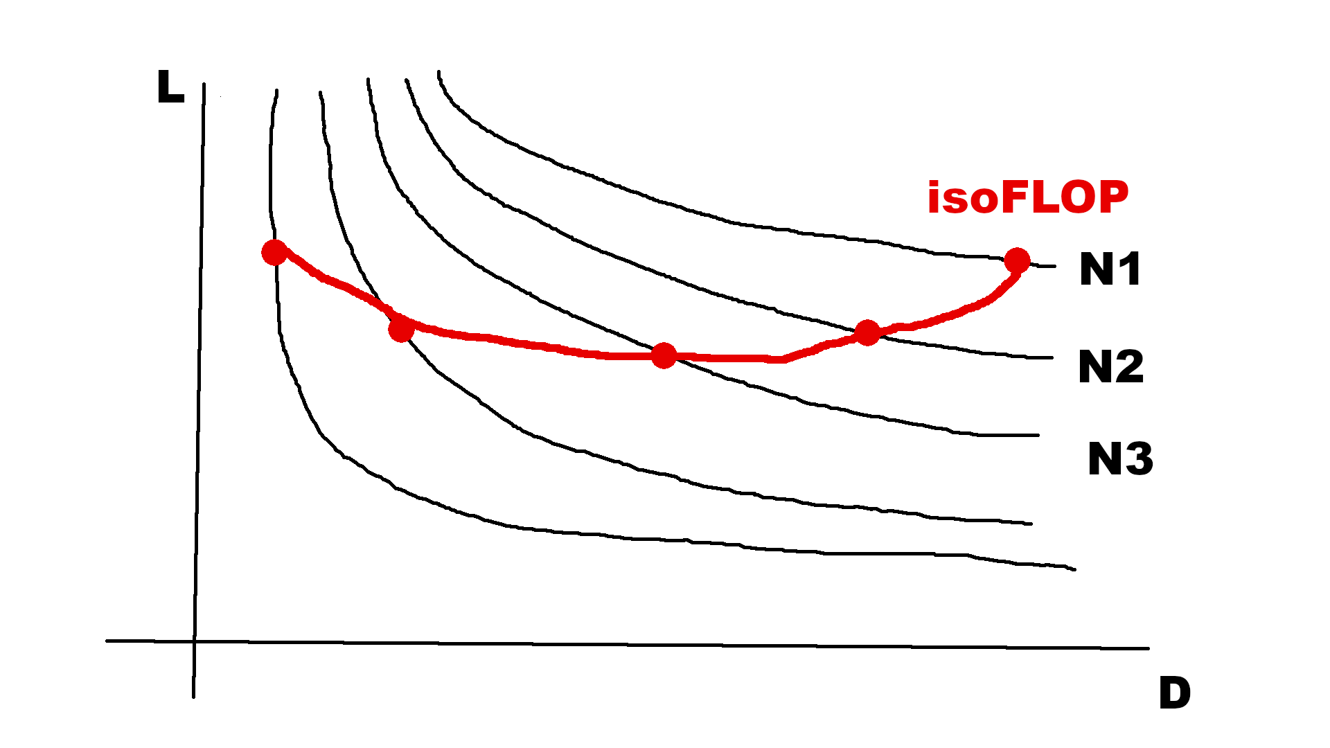
The curve that you plot above is not a scaling law, because we consider a limited compute budget: a scaling law must be able to scale, which requires an increasing compute budget. This is why scaling laws are often plotted with the compute on the X axis. When you fix the compute budget C, you should try and find the compute-optimal model, i.e., which number of parameters N and data D give the lowest loss? To find it, you can train various (N,D) for the same C: this boils down fixing N1 and training with as much D as possible allowed by C. Then increasing N2, and train again for as long as possible, etc. You obtain minimal losses for N1, N2… You can plot this isoFLOP curve: the minimum of the isoFLOP curve is the compute-optimal model.

The scaling law is then the loss obtained by this compute-optimal model when increasing C.