Best practices
- A few hints:
- design the model
- hyper-parms tuning
- prepare data
- design experiments
- Focus: contrastive, CLIP, diffusion
- Pytorch new: lightning
- Prepare exercice right now: run:
from transformers import CLIPProcessor, CLIPModel, CLIPTokenizer
from PIL import Image

model = CLIPModel.from_pretrained("openai/clip-vit-base-patch32")
processor = CLIPProcessor.from_pretrained("openai/clip-vit-base-patch32")
Best practices: design the model
Choice of module’s topology
- Depends on data
- Rely on standard practices
- Keep in mind the properties of each layer type
- More and more: combination of modules
- Use freedom to plug-in various components/losses
- Always optimize globally (E2E)
- ex: CNN+RNN+attention
Choice of loss
- Go beyond simple loss:
- you may combine conflicting objectives
- you may add constraints
- ex: you’re interested in predicting weather cycles
- add a sinus parameter parallel to your RNN
- loss matches long-term sinus + short-term RNN
- But don’t start straight with a complex toplogy/loss:
- start simple, experiment
- identify limits
- progressively add components/losses
Devil’s in the details: control variance
- Objective: scale at the input of the layer \(\simeq\) scale at its output
- Otherwise, some neurons will dominate others
- Assume \(x\sim N(0,\sigma)\) with constraints \(\sum w_i=0\) and \(\sum w_i^2=1\); then, with the linear layer, \(E[y]=0\) and \(E[y^2]=\sigma^2\).
- after ReLU, variance approx. divided by 3, so you may replace ReLU with \(\sqrt 3 relu(y)\)
- see Caltech course
Non-differentability
- Avoid non-differentiable functions
- But can be used when necessary:
- sampling: reparameterization trick
- step-like: REINFORCE
- algorithms/logic/sorting…: diff. expectation
- see “Learning with Differentiable Algorithms”
Best practices: hyper-parameter tuning
From very complex…
- Auto-ML
- Neural Architecture Search
- But NAS evaluation is frustratingly hard
- Lindauer & Hutter’s NAS best practices checklist
Best practices for reporting reproducibility
- For all experiments, report code
- code of training pipeline
- code for search space
- hyperparms used + random seeds
- code for NAS method
- hyperparms of NAS method + random seeds
- When comparing, check
- same dataset, split, search space, code, hyperparms
- for confounding factors (hardware, libs versions…)
- run ablation studies
- same evaluation protocols
- performance over time
- compare to random search
- multiple runs and report seeds
- When reporting
- how hyperparms tuned, what time and resources
- time for entire E2E method
- report all details of XP setup
To moderately complex…
- Bayesian optimization
- Evolutionary optimization
- Population based
… to simple ones
- Random Search
- Grid Search
- “Graduate student descent” is still the best!
Devil’s in the details: batch size
- If batch = corpus: classical Gradient Descent
- If batch = 1: stochastic Gradient Descent
- Smaller batch => more regularization
- Larger batch => faster parallelization (GPU)
- Pratical values:
- Standard size models: batch = 32, …, 128
- Large LLM: batch = 1024, 2048…
- Optimal batch size for transformers, from:
\(\left( \frac S {S_{min}} -1 \right) \left( \frac E {E_{min}} -1 \right) = 1\)
- \(S_{min}=\)nb of steps needed to reach target loss \(L\)
- \(B=\) batch, \(S=\) training steps, \(E=BS=\) data samples
- critical batch size: \(B_c(L)=\frac{E_{min}}{S_{min}}\)
- for transformers: \(B_c(L) \simeq \frac {B_*} {L^{1/{\alpha_B}}}\)
- \(B_* \simeq 2\times 10^8\) and \(\alpha_B \simeq 0.21\)
- Don’t forget: tune LR first!
Best practices: prepare data
- Deep Learning is End-to-End:
- no need to compute smart features from data
- as long as there is enough data!
- otherwise, use classical ML: converges faster
- Tip1: don’t use deep learning with few data, except when transfer learning is an option
- Tip2: randomize your training corpus
- Tip3: normalization everywhere
- input and output data
- between layers
- within batches
Manual annotations
- manual annotation = very costly, do not scale
- not a problem any more with scale:
- Transfer learning, finetuning
- Zero-shot learning, few-shot learning
- manually annotating (few) data also very useful for finetuning,
adapting, improving the model
- but it shall be done as a complement of the main training phase
- Tip4: always try to exploit unlabeled data
Data augmentation
- often very useful:
- augment your training corpus
- easy way to model uncertainty
- increase model’s robustness
- but requires to carefully think about how to augment
Best practices: design experiments
- 10% of time for writing code
- 90% of time for running experiments
- run, analyze, modify
- loop
- XP phase 1: 80% of human time
- iterate quickly with short cycles until confident
- XP phase 2: 80% of machine time
- script, scale, deploy on cluster
- First, create an evaluation corpus
- Then, create a training corpus
- warning: overlap with evaluation corpus
- think twice: how do you want your model to generalize?
- Finally, create a development corpus
- avoid cross-validation if not absolutely required!
- Always track the training loss + development loss curves!
- use easy tools for that: lightning + tensorboard
- track variability of resuts
- rerun multiple times with random init, with other data:
- if variability too large: red flag!
- if variability too low: red flag!
- rerun multiple times with random init, with other data:
- Beware too good results:
- accuracy=99%: red flag! (test contamination, ill-posed pb…)
- accuracy=2%: don’t worry! (bug, bad data, bug, bug…)
- Never stop at one metric!
- look at predictions, in various cases
- be creative, use other metrics
- Don’t be too optimistic, be ultra-cautious, be doubtful
- Always keep a safe doubt about your results:
- there are always bugs hiding somewhere!
- Always Keep on tracking bugs, until the very end!
- Progressively increase trust in your code; XP after XP:
- you build up a mental model of your model
- you better understand its weaknesses, edge cases
- When you trust is high enough, release
- Progressively increase trust in your code; XP after XP:
- Try to overfit on one batch
- once you know where the “overfitting point” is, you can:
- scale: linear relation btw parameters / dataset size
- decide: scale and stay a bit below the “overfitting point”
- or try overparameterized regime (risky!)
- if you have the choice: add more data, or iterate more
- always add more data: it’s always better!
- ideally: a single epoch over as much data as possible
- When finetuning, beware of catastrophic forgetting!
- Always start by designin a clear evaluation protocol
- Iterate very quickly (initially: a few minutes max per training)
- small model, small data
- runs many experiments
- automate the whole process
- Once you’re really confident about your process, start to scale
Contrastive training
Classification vs. metric learning
- Ex: a person = (height, weight, gender, salary…)
- Who are the most similar?
- Ex: 3 photos of cars from different angles; 2 are from the same car
- We want the distance btw them to be small
- metric learning: train a model to compute dist(a,b)
- Use cases:
- Instance-based learning
- Prototype networks / K-NN
- Ranking
- Large number of classes…
- Either learn a distance: \(d(x,y) = s(x,y) = f_{\theta}(x,y)\)
- Or use a standard distance and learn a representation: \(e(x) = f_{\theta}(x)\) \(d(x,y) = e(x) \cdot e(y)\)
- How to train such a model?
- Regression:
- Train to predict gold truth distance \(d(x,y)\):
- Too hard (requires lots of samples, precise prior knowledge)
- How to train such a model?
- Ranking loss!
- Train the model to make similar examples closer and dissimilar examples farther apart
- See blog
Pairwise ranking loss

- Trained E2E with loss:
\(L = \Big\{ {\begin{matrix} d(f_{\theta}(x_a),f_{\theta}(x_p)) ~~~~ if ~~ pos\\ \max(0,m-d(f_{\theta}(x_a),f_{\theta}(x_n)) ~~~~ if ~~ neg \end{matrix}}\)
- margin \(m\): don’t loose efforts training already far negative pairs
Triplet ranking loss

\[L = \max\left(0,m+d(f_{\theta}(x_a),f_{\theta}(x_p))-d(f_{\theta}(x_a),f_{\theta}(x_n))\right)\]
- Easy triplet: \(d(f_{\theta}(x_a),f_{\theta}(x_p)) >
d(f_{\theta}(x_a),f_{\theta}(x_n))+m\)
- \(L=0\), parameters not updated
- Hard triplet: \(d(f_{\theta}(x_a),f_{\theta}(x_p)) <
d(f_{\theta}(x_a),f_{\theta}(x_n))\)
- \(L>m>0\)
- Semi-hard triplet: \(d(f_{\theta}(x_a),f_{\theta}(x_p)) <
d(f_{\theta}(x_a),f_{\theta}(x_n)) <
d(f_{\theta}(x_a),f_{\theta}(x_p))+m\)
- \(0<L<m\)
Typical model: Siamese net
- In image recognition
- Same/shared CNN computes representation of anchor/pos/neg images
- Pairwise ranking loss: \[L = y||f(x_a)-f(x_p)|| + (1-y)\max(0,m-||f(x_a)-f(x_n)||)\]
Typical model: Triplet net
- In image recognition
- Same/shared CNN computes representation of anchor/pos/neg images
- Triplet ranking loss: \[L = \max(0,m+||f(x_a)-f(x_p)||-||f(x_a)-f(x_n)||)\]
Negative sampling
- Training procedure:
- Sample anchor
- Sample positive example
- Sample negative example : critical!
Negative sampling
- Nb of possible pairs = \(O(n^2)\)
- good for few-shot
- otherwise, you have to choose!
- Sampling easy triplets = no training occur
- Sampling hard triplets = erratic convergence
- Sampling semi-hard triplets = good!
Unsupervised setting
- Positive samples may be obtained by data augmentation:
- rotate, scale, crop images
- mixing (hard negative) images to control difficulty
Ranking vs. Cross-ent loss
(see github blog)
- Train ConvNet on MNIST with 10-class cross-entropy loss
- Extract 2-dim embeddings from penultimate layer:
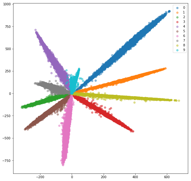
- Distance btw classes not good
- Train a siamese net
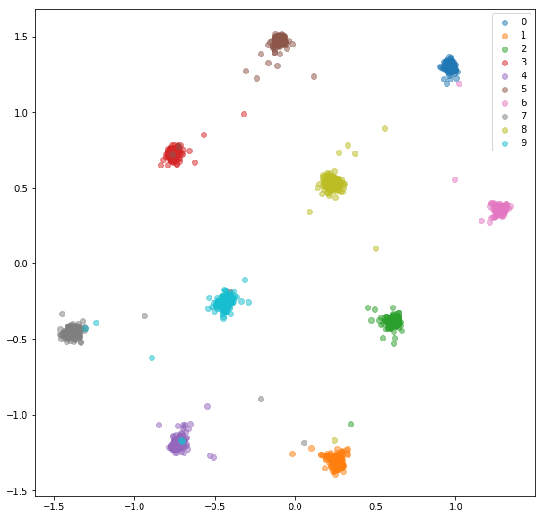
- Distance btw classes are good
- Train a triplet net
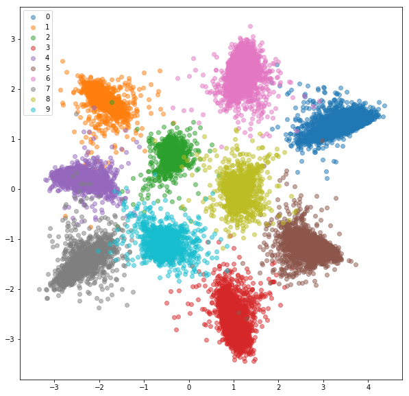
- Didn’t train for same-class embed. get closer, but trained for same class embed. to be closer than inter-class embed.
Other advantages of ranking loss
- Cross-Ent loss not robust to noisy labels
- Many classes are costly with softmax
- Meaningful dist btw embeddings is desirable (S-BERT)
- see Lilianweng blog
1-shot/few-shot learning
- You have an image dataset \(T\) with \(N\) classes
- You add 1 new class with 1 example \(x_0\) only \(\rightarrow T' = T \cup \{x_0\}\)
- Contrastive training on \(T\)
- New unknown sample \(x\):
- Compute \(d(f(x),f(x_0))\) and compare to \(d(f(x),f(x_1))\)…
In pytorch
- CosineEmbeddingLoss = pairwise loss with cosine dist
- MarginRankingLoss = pairwise loss with euclidian dist
- TripletMarginLoss = triplet loss with euclidian dist
Extension: Multi-class N-pair loss (Sohn, 2016)
- one anchor, one pos, \(N-1\) neg \[L = \log\left( 1+\sum_{i=1}^{N-1} \exp(f(x_a) \cdot f({x_n}_i) - f(x_a) \cdot f(x_p)) \right)\]
- With 1 ex. per class, equivalent to softmax
Practice: triplet loss
- Goal: train a linear embedding space with triplet loss
- Synthetic data:
- scalar input, 2 classes \(c\in \{0,1\}\)
- \(x|c \sim N(\mu_c,\sigma_c=0.1)\)
- Embedding dim = 5
- lightning = pytorch library that
- automates cpu/gpu runtime
- simplifies training loop
- generates tensorboard logs
- pytorch lightning in practice:
- replace and extend nn.Module:
import pytorch_lightning as pl

class Mod(pl.LightningModule):
    def __init__(self):
        super().__init__()
        self.W = torch.nn.Linear(1,5)

    def configure_optimizers(self):
        opt = torch.optim.AdamW(self.parameters(), lr = 1e-3)
        return opt

    def training_step(self, batch, batch_idx):
        anc, pos, neg = batch
        ea = self.W(anc)
        ep = self.W(pos)
        en = self.W(neg)
        dp = torch.nn.functional.triplet_margin_loss(ea,ep,en)
        self.log("train_loss", dp, on_step=False, on_epoch=True)
return dp- you need a dataset that generates anchors/pos/neg:
class TripDS(torch.utils.data.Dataset):
    def __init__(self):
        super().__init__()

    def __len__(self):
        return 1000

    def __getitem__(self,i):
        if i%2==0:
            # pair: on sample une ancre from class 1
            xa = torch.randn(1)/10.-0.5
            xp = torch.randn(1)/10.-0.5
            xn = torch.randn(1)/10.+0.5
            return xa,xp,xn
        else:
            # impair: on sample une ancre from class 2
            xa = torch.randn(1)/10.+0.5
            xp = torch.randn(1)/10.+0.5
            xn = torch.randn(1)/10.-0.5
return xa,xp,xn- Train:
traindata = TripDS()
trainloader = torch.utils.data.DataLoader(traindata, batch_size=1, shuffle=False)
mod = Mod()
logger = pl.loggers.TensorBoardLogger(save_dir="logs/", flush_secs=1)
trainer = pl.Trainer(limit_train_batches=1.0, max_epochs=1000, log_every_n_steps=1,logger=logger)
trainer.fit(model=mod, train_dataloaders=trainloader)- TODO:
- run this training and observe the logs with:
tensorboard --logdir=lightning_logs/- does it converge?
- how could you do hard negative sampling?
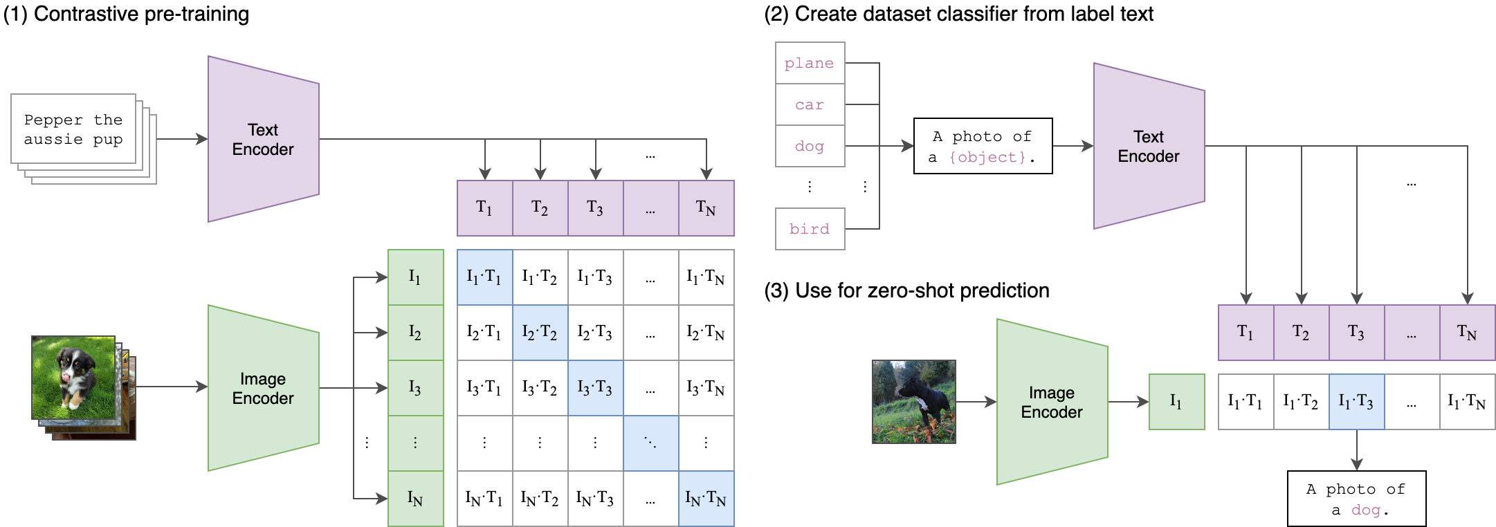
CLIP model
- CLIP is a model that builds a joint text/image embedding space
- uses 2 transformers, resp. for image and text + cosine dist
- It is trained with a ranking loss: multi-class N-pair loss
- they show that ranking loss much faster to train
- Given an input image and several texts, it outputs similarity scores
- How to use it:
from transformers import CLIPProcessor, CLIPModel, CLIPTokenizer
from PIL import Image

model = CLIPModel.from_pretrained("openai/clip-vit-base-patch32")
processor = CLIPProcessor.from_pretrained("openai/clip-vit-base-patch32")
image = Image.open("difftrain.png")
inputs = processor(text=["a rabbit","a curve","a chair"], images=image, return_tensors="pt", padding=True)
outputs = model(**inputs)
logits_per_image = outputs.logits_per_image  # this is the image-text similarity score
probs = logits_per_image.softmax(dim=1) # we can take the softmax to get the label probabilities- Practice: try it with your own image and texts
- Generative use?
- CLIP can tell whether texts == images
- TODO: could you generate an image, just with CLIP?
Diffusion models
Prepare
- install diffusers with conda or pip
- create an account + token at huggingface
- login locally with: huggingface-cli login
- download stable diffusion model (5GB):
from diffusers import StableDiffusionPipeline
pipe = StableDiffusionPipeline.from_pretrained("CompVis/stable-diffusion-v1-4", use_auth_token=True)
References
- https://lilianweng.github.io/posts/2021-07-11-diffusion-models/
- https://ayandas.me/blog-tut/2021/12/04/diffusion-prob-models.html
- https://huggingface.co/blog/annotated-diffusion
- A diffusion process transforms a complex distribution ($p(x) = $set of real images) into a simple distribution (N(0,1))
- This transformation can be modeled through a Markov Chain, i.e., the repeated application of a transition kernel: \[x_t \sim q(x|x_{t-1})\]
- The Markov Chain eventually converges towards its stationary distribution: \(x_\infty \sim p_{prior}\)
- in practice, we keep \(x_T\) with \(T\) large enough (1000)

- Gaussian diffusion:
- We choose \(p_{prior} = N(0,I)\) and \[q(x_t|x_{t-1}) = N(x_t;\sqrt{1-\beta_t} x_{t-1},\beta_t I)\]
- \(\beta_t \in R\) is a decaying schedule
- Stochastic forward diffusion:
- sample \(x_0 \sim p_{data}\)
- compute \(x_T \sim N(0,I)\)
- Stochastic reverse diffusion:
- sample \(x_T \sim N(0,I)\)
- compute \(x_0 \sim p_{data}\)
- also assumed gaussian: \[p_\theta(x_{t-1}|x_t)=N(x_{t-1};\mu_\theta(x_t,t),\Sigma_\theta(x_t,t))\]
- modeled by a DNN with \(\theta\) trained from data
- It’s a generative model, just like GAN, VAE
- reverse diffusion process modeled by a DNN that is trained to gradually denoise an image from pure noise
- Training objective: minimize negative log-likelihood: \[L=E_{x_0\sim p_{data}}[-\log p_\theta(x_0)]\]
- Hard to minimize (depends on \(T\) random variables), so we minimize its upper bound:
\[L\leq E_{x_0\sim p_{data},x_{1:T}\sim q(x_{1:T}|x_0)}\left[-\log p(x_T)-\sum_{t\geq 1} \log \frac {p_\theta(x_{t-1}|x_t)}{q(x_t|x_{t-1})}\right]\]
- sampling a \(x_{1:T}\sim q(\cdot|x_0)\) boils down running a forward pass
- all quantities are tractable and closed form
- Reparameterization: our DNN can predict the noise instead of predicting the Gaussian parameters: \[\epsilon_\theta(x_t,t)\]
- We can sample and directly compute any \[x_t = \sqrt{\bar \alpha_t}x_0 + \sqrt{1-\bar \alpha_t}\epsilon\] with \(\alpha_t = 1-\beta_t\) and \(\bar\alpha_t = \prod_{s=1}^t \alpha_s\)
- The loss is now the simple MSE: \[L=||\epsilon - \epsilon_\theta(x_t,t)||^2\]

In practice
from diffusers import StableDiffusionPipeline
pipe = StableDiffusionPipeline.from_pretrained("CompVis/stable-diffusion-v1-4", use_auth_token=True)
prompt = "a photo of cat playing with a rat"
image = pipe(prompt, guidance_scale=7.5).images[0]
image.save("cat.png")- requires 16GB of RAM
- TODO: try to generate an image from any prompt
Best practices: reduce costs
Reducing costs: softmax
- softmax: \(O(n)\)
- costly with many classes
- requires a large network
- hierarchical softmax: \(O(\log n)\)
- sampling-based approximate softmax
- contrastive loss
Reducing costs: embedded models
- Sharing models across pytorch, keras, tensorflow, JAX: ONNX format
- in browser: tensorflow-js, ONNX.js
Reducing costs: mixture of experts
- \(N\) experts, \(1\) gate
- gate = hard softmax
- data flows into only \(1/N\) or \(p/N\) experts
- reduce costs or increase size?
- GShard model
Reducing costs: pruning
- after training a big model, prune “useless” parameters
- Ex: remove neurons rarely activated
- good task performances when removing up to 90% or parameters!
- “lottery ticket hypothesis”
- but genericity?
Reducing costs: NAS
- Network Architecture Search
- combination of growing + pruning
- “firefly neural networks”
Reducing costs: distillation
- Once a big model is trained, create a small model
- Train the small model (student) to reproduce the logits of the big model (teacher)
Reducing costs: quantization
- on CPU, pytorch supports only float32
- on GPU, pytorch supports float16 (and bfloat16)
- integer quantization (see bitsandbytes)
- int8(): studies the distrib of float values, discretize
- int4(): rare
- bit
Reducing costs: parallelization
- GPU = parallelizes tensor operations
- How to parallelize on multiple GPU?
- Data parallelization:
- copy model onto each GPU
- split data across GPUs
- train locally
- regularly merge gradients (synchronously or asynchronously, cf. Hogwild)
- Model parallelism:
- put one layer on each GPU
- data flows from one GPU to another
- useful for very large models
- Pipeline parallelism:
- same as model parallelization
- but continuously feeds in samples
- no idle GPU!
- Federated learning:
- copy model into “far away” nodes
- keep data local (private) per node
- train locally
- aggregate local gradients into central model
- redistribute global parameters
- Diff with distributed computing:
- slow transmission in FedL
- so compromise btw local training & aggregation
- If aggregate at every step == distributed computing
- If aggregate only at the end == ensembling
- FedL preserves privacy/copyright:
- local data never leaves each node
- but gradients can be attacked
- but central model can be attacked
- see membership inference attacks, data extraction attacks, model inversion attacks…
- So FedL may be combined with:
- Differential Privacy
- add noise to “hide” training samples in parameters
- Secure Multiparty Computation
- gradients are encrypted
- Differential Privacy
- Convergence of Machine Learning and Security domains
- Other problems: malevolent/unreliable nodes?
- FedL related to
- ensembling
- voluntary computing
- collaborative computing
- Most famous applications of FedL:
- Hospitals data
- Google android: next word prediction
Reducing costs: memory issues
- Libraries: deepspeed, accelerate
- Avoid redundancy across GPUs
- Compromise during training btw:
- save intermediary matrices vs.
- recompute them
- same for computation graph
- Offloading:
- When GPU memory full, move non-urgent parms into CPU RAM
- When RAM full, move non-urgent parms into disks
- NVMe disks extremely useful!
- In practice: choice of a library:
- transformers lightning
- transformers accelerate
- deepspeed
- fairseq
- megatron
- MosaicML
Best practices: generating sequences
Auto-regression
- Typical of LSTM, seq2seq, but even MLP or any causal network!
- Causal models: \(p(x_t|x_0,\dots,x_{t-1})\)
- sample \(\hat x_t \sim p(x_t|x_0,\dots,x_{t-1})\)
- complete the current sequence: \(x_0,\dots,x_{t-1},\hat x_t\)
- iterate
- PB1: hard to parallelize!
- Iterative refinement/diffusion
- PB2: error propagate
- greedy/beamsearch/A*
- PB3: mismatch training process vs. test process
- teacher/student/professor forcing
- Greedy decoding
- choose \(\hat x_t = \max_x p(x|x_0,\dots,x_{t-1})\)
- typically used in LSTM & all autoregressive models
- replaced by sampling when you want variability
- not globally optimal
- Ex prediction: “le président de … dirige la SPA …”
- Greedy: “le président de la république”
- but given SPA farther: “le président de l’association”
- Globally optimal decoding:
- Try every possible continuation: \(O(V^T)\)
- With specific simplifying assumptions: Dijkstra, …
- Most famous, with \(p(x_t|x_{t-1})\): Viterbi: \(O(VT)\)
- Approximate globally optimal decoding:
- A*,…
- beam search: keep a list of the \(N\) best continuations at any time
- And for training?
- CTC loss: equivalent for DNN of the Baum-Welch algorithm for Markov Chains
- Mostly used in OCR, or when segmentation is unknown
- PB3: mismatch training process vs. test process
- teacher/student/professor forcing
- Teacher forcing:
- Use gold \(x_0,\dots,x_{t-1}\) to train \(p(x_t|x_0,\dots,x_{t-1})\)
- Student forcing:
- Use predicted \(\hat x_0,\dots,\hat x_{t-1}\) to train \(p(x_t|x_0,\dots,x_{t-1})\)
- Professor forcing:

Diffusion
- Diffusion instead of auto-regression
- Diffusion-LM: https://arxiv.org/abs/2205.14217
- DiffuSeq: https://arxiv.org/abs/2210.08933
- Diffsound: https://arxiv.org/abs/2207.09983