• Overview:
  • Reminder of Bayesian inference
  • Uncertainty at the output of DNN
  • Uncertainty in latent layer
  • Bayesian Neural Networks
• refs:
  • https://www.youtube.com/watch?app=desktop&v=lhwk4ESlyMA&feature=youtu.be

• Goal1: compute how reliable the model output is
  • we know the output of MLP classifier = \(p(y|x)\)
  • but we know it overestimates the probability of its prediction
• Better method: conformal prediction sets
  • paper
  • use a held-out dataset to estimate proba that model is correct
  • for any target confidence, returns a set of possible labels

Bayes vs. DNNs

• Basic DNNs do not consider the process that generates data:
  • They consider only fixed-point data samples
  • Given one point \(x\), they compute one output \(y\)

• Exemple:
  • inputs = day, month, location
  • output = temperature
• A fixed point is not enough: there’s a lot of variability
  • wind, previous weather in neighbouring places…
• We’d prefer mean + stdev

• 1st source of uncertainty:
  • many factors are unknown
• 2nd source of uncertainty:
  • our model is limited
  • ex: input = history + geo-grid of T°,P,W,rain,lum
  • output still erronous

• Bayesian networks
  • model the distribution of \(y\) given \(x\)
  • Get uncertainty of the prediction
  • Enable sampling various good outputs
  • You may include prior knowledge
    • e.g., T° increase over years because of global warming

• But BN are
  • less powerful than DNNs
  • very costly to train (in general)
• Can we do the same with DNNs ?

Brief reminder of Bayesian models

• Bayesian models assume all vars are generated from a process:
  • Variable \(X\) is sampled from a distribution, which is usually assumed parametric: \[X \sim Mult(\theta)\]
  • \(\theta\) usually trained with MLE, MAP or Bayesien inference

• Maximum Likelihood
  • maximum likelihood <=> cross-entropy
  • data follow a true distribution \(P^*(X)\), approximated by parametric distrib \(P(X;\theta)\)
  • MLE: \(\theta^* = \arg\max_\theta P(X;\theta)\)

• Assume iid samples:
  • \(\theta^* = \arg\max_\theta \prod_i P(X_i;\theta) = \arg\max_\theta \sum_i \log P(X_i;\theta)\)
  • \(\theta^* = \arg\min_\theta E_{X \sim P^*(X)} \left[\log \frac 1 {P(X;\theta)} \right]\)
  • which is the equation of the cross-entropy

Limits of Maximum Likelihood

• Only relies on the evidence
• Does not take into account prior knowledge
• but why bother about priors?

• Ex: we know that, in July, T° is usually positive
• MLE will “rediscover” this fact through data
  • bad use of evidence / training time
  • much more efficient to tell it beforehand
• Prior knowledge makes better use of few data

• Bayesian models assume that we have some knowledge about the distribution before observing anything
  • prior distribution \(P(\theta)\)
  • Now \(\theta\) is a random variable !
  • If the prior knowledge is good enough, then we don’t need data at all

• Combining prior knowledge + data: (1)
  • We want to find the best \(\theta\) according to both prior and likelihood
  • maximum a posteriori: \(\max_\theta P(\theta|X) = \max_\theta P(X|\theta) P(\theta)\)
  • L2 regularization <=> MAP with a Gaussian prior on the weights

• Combining prior knowledge + data: (2)
• Estimate the full posterior: observations (evidence) come in to modify this prior belief:
  • Transforms the prior \(P(\theta)\) into the posterior \(P(\theta|X)\)
  • = Bayesian Inference

SGD == Approx. Bayesian Inference

https://arxiv.org/abs/1704.04289

• constant-rate SGD simulates a Markov chain with a stationary distrib
• possible to adjust the LR of constant SGD to best match the stationary distrib to a posterior

Distributions in DNNs

• If we use a vanilla DNN, do we have any information about the distribution of possible outputs?
• How can we modify the vanilla DNN to get more information?

• Vanilla DNN:
  • Can we measure uncertainty of the output?
• DNN that outputs a distribution (Mixture Density Network)
• DNN with a latent Random Variable
  • RBM, DBN
  • VAE
• Bayesian DNN

Can we still get a distribution out of a vanilla DNN ?

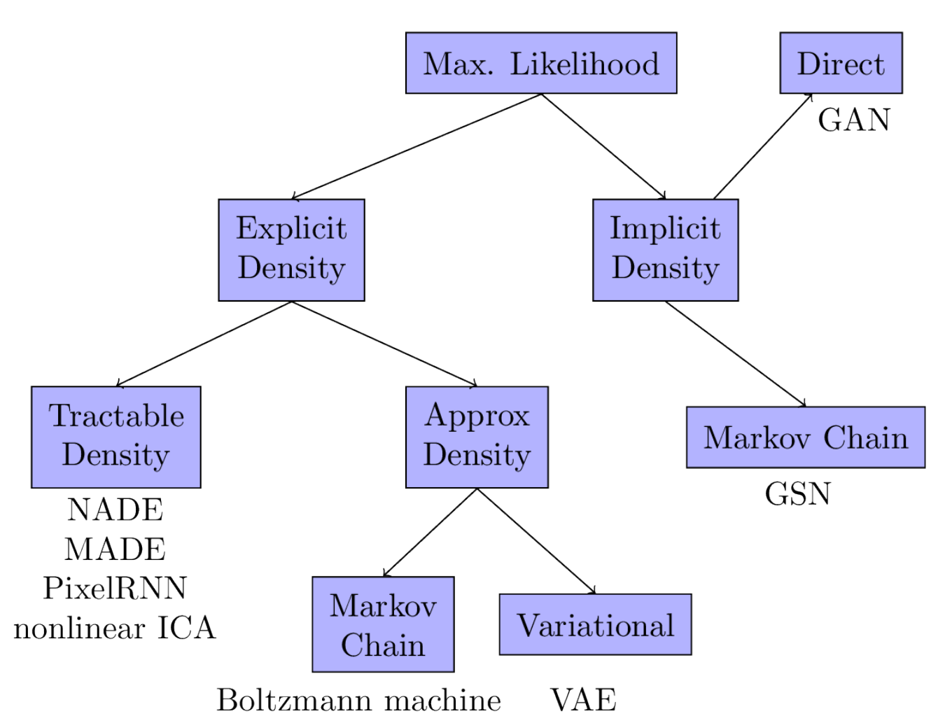
• Famous examples: generative model:
  • A generative model samples from a density of probability
  • VAE: the latent \(z\) is randomly sampled from a Gaussian distribution
  • GAN: the generator is fed with a random input

Softmax approximates posterior

• Multi-class classification:
  • Objective = classify an input \(x\)
    • e.g., does an utterance express joy, anger, sadness… ?
    • Celebs pictures: who is she/he ?
  • One output neuron per class
    • each output neuron gives a score (logits)
    • normalized by softmax –> probability
    • … which probability ?

• (Bishop,94) proves that a MLP trained with cross-entropy (and infinite data) approximates the posterior \(P(y|x)\)
• But in practice, not very reliable to estimate uncertainty
  • Gal & Ghahramani (2016) show that a model can be uncertain in its predictions even with a high softmax output.
  • Calibration
• Bishop proposed another analysis to estimate output distrib with MSE

Gaussian approximation

(Bishop94):

• assume infinite data \((x,y)\), a DNN \(f(\cdot;\theta)\); the MSE error is:

\[\int \int (f(x;\theta) - y)^2 p(x,y) dx dy\]

\[(f(x;\theta) - y)^2 = (f(x;\theta) - y + E[y|x] - E[y|x])^2\]

\[\begin{eqnarray} (f(x;\theta) - y)^2 &=& (f(x;\theta) - E[y|x])^2 + (E[y|x]-y)^2 + \\ && 2(f(x;\theta) - E[y|x])(E[y|x]-y) \end{eqnarray}\]

\[\begin{eqnarray} (f(x;\theta) - y)^2 &=& (f(x;\theta) - E[y|x])^2 + E[y|x]^2 + y^2 -2E[y|x]y +\\ && 2f(x;\theta)E[y|x] -2f(x;\theta)y - 2E[y|x]^2 + 2E[y|x]y \end{eqnarray}\]

\[\begin{eqnarray} (f(x;\theta) - y)^2 &=& (f(x;\theta) - E[y|x])^2 + y^2 + 2f(x;\theta)E[y|x] - \\ && 2f(x;\theta)y -E[y|x]^2 \end{eqnarray}\]

Consider the first term in \(2f(x;\theta)...\) into the integral:

\[\begin{eqnarray} \int 2f(x;\theta)E[y|x] p(y|x)p(x) dy &=& 2f(x;\theta) p(x) \int E[y|x] p(y|x) dy \\ &=& 2f(x;\theta) E[y|x] p(x) \end{eqnarray}\]

for the other term: \[\begin{eqnarray} \int 2f(x;\theta)y p(y|x)p(x)dy &=& 2f(x;\theta) p(x) \int y p(y|x)dy \\ &=& 2f(x;\theta) E[y|x] p(x) \end{eqnarray}\]

so \[\begin{eqnarray} \int (f(x;\theta) - y)^2 p(x,y)dy &=& p(x)(f(x;\theta) - E[y|x])^2 +\\ && p(x)(E[y^2|x] - E[y|x]^2) \end{eqnarray}\]

so the MSE error is \[\int (f(x;\theta) - E[y|x])^2 p(x)dx + \int (E[y^2|x] - E[y|x]^2)p(x)dx\]

The MSE error only depends on the model parameters through the first term, and it is minimum when \(f(x;\theta) = E[y|x]\)

• Consequently, if we want to model uncertainty of the DNN output with a Gaussian, we can interpret that, after training, the DNN:
  • outputs the expected value (mean)
  • The variance of the error (=uncertainty) can be computed from the corpus (second term)

• OK, we have way to estimate the uncertainty from the corpus
• but can we let the DNN computes it itself ?

Gaussian mixture approximation

• (Bishop, 94) proposes the “Mixture Density Network”:
  • the input X is passed into an MLP with 3 outputs:
    • \(K\) mixing values \(\alpha\), which are further passed into a softmax
    • \(K\) means \(\mu\)
    • \(K\) variances \(\sigma\), which are further passed into some positive-only function

• the final output of the model is a mixture of Gaussians: \(\sum_k \alpha_k N(x;\mu_k,\sigma_k)\)
  • The output is a probability distribution that represents the possible values of \(y\) given \(x\)
  • So if you want just one value \(y\), you have to sample
• See Bishop’s report on MDN

DNNs with latent random variable

• We have seen how to model the parameters of a GMM with a DNN
• It is possible to model parametric distributions inside a DNN, but only for a Gaussian.
• This may seem very limited, but the following DNN layers may transform this Gaussian into any other distribution!

VAE

• Explicitly model a distribution
• Encoder transforms input \(x\) into a distribution \(p(z)\sim N(\mu,\sigma)\)
• Decoder transforms a sample \(z\sim p(z)\) into the output \(\hat x\)

• We want to train the VAE with MLE, but the likelihood is hard to compute: \[\log p(x) = \log \int p(z)p(x|z)dz\]

• variational principle:
  • convert difficult computation into optim. problem
  • we chose a variational family \(q(z|x) \in Q\)
• How to get the ELBO (Evidence Lower BOund): \[\log p(x) = \log \int \frac {q(z|x)}{q(z|x)}p(x,z)dz = \log E_q \frac {p(x,z)}{q(z|x)}\]
  • the log of a sum is not easy to differentiate…

• Much better to get the sum of the log:
• Jensen’s inequality gives the ELBO: \[\geq E_{q(z|x)} \log \frac {p(x,z)}{q(z|x)}\]

• Note: when we maximize the lower bound, we actually make \(q\) closer to \(p\): \[\max_q E_{q(z|x)} \log \frac {p(x,z)}{q(z|x)} = \log p(x) - \min_q D(q(z|x)||p(z|x))\]

• So MLE involves now a double optimization (\(\hat p\) is the empirical corpus): \[\max_{p,q} E_{\hat p(x)}E_{q(z|x)} \log \frac {p(x,z)}{q(z|x)}\]

• Let us consider encoder parameters \(\phi\) and decoder parameters \(\theta\) \[\max_{\theta,\phi} E_{\hat p(x)}E_{q_\phi(z|x)} \log \frac {p(z)p_\theta(x|z)}{q_\phi(z|x)}\]

• SGD involves computing \[\nabla_\phi E_{q_\phi(z|x)} \log \frac {p(z)p_\theta(x|z)}{q_\phi(z|x)}\]

  • hard: cannot be expressed as an expected value of a gradient
  • let’s make it not dependent on \(\phi\): reparameterization trick

• Instead of sampling from \(q\), we sample from a fixed distribution \(p(\epsilon)\): \[\nabla_\phi E_{q_\phi(z|x)} \log \frac {p(z)p_\theta(x|z)}{q_\phi(z|x)} = \nabla_\phi E_{p(\epsilon)} \log \frac {p(T(\epsilon))p_\theta(x|T(\epsilon))}{q_\phi(T(\epsilon)|x)}\]

• which is possible when \(q_\phi(z|x)\) is a conditional diagonal Gaussian model with: \[p(\epsilon)=N(0,1)\] \[T(\epsilon)=\mu_\phi(x) + \epsilon \cdot \sigma_\phi(x)\]

• We now have: \[\nabla_\phi E_{p(\epsilon)} \log \frac {p(T(\epsilon))p_\theta(x|T(\epsilon))}{q_\phi(T(\epsilon)|x)}= E_{p(\epsilon)} \nabla_\phi \log \frac {p(T(\epsilon))p_\theta(x|T(\epsilon))}{q_\phi(T(\epsilon)|x)}\]
• can be estimated with Monte Carlo!

In practice

• given \(x\), the encoder computes \(\mu_\phi(x)\) and \(\sigma_\phi(x)\)
• sample an \(\epsilon \sim N(0,1)\)
• build the latent representation \(z=\mu_\phi(x) + \epsilon \cdot \sigma_\phi(x)\)
• pass \(z\) to the decoder \(\hat x = p_\theta(x|z)\)
• optimize sum of:
  • standard loss (MSE, cross-ent) for \(\theta\): \(l(\hat x, x)\)
  • regularizer for \(\phi\): \(KL(q_\phi(z|x)||N(0,1))\)

• and for a given \(x\): \[KL(q_\phi(z|x)||N(0,1))= \mathbb{KL}\left( \mathcal{N}(\mu, \sigma) \parallel \mathcal{N}(0, 1) \right)\] \[ = \sigma^2 + \mu^2 - \log \sigma - \frac{1}{2}\]

• Ref: probabilistic view of VAE
• Ref: backprop in sampling net

General pb: non-diff

• Doubly stochastic system:
  • stochastic component: sampling in the DNN
  • stochastic optimization: sampling a batch in SGD
• Let’s define \(\hat x \sim p_\theta(x)\) the (random) output of the DNN
• \(f\) is the loss fct, we can estimate the expected loss with MC: \[E_{p_\theta}[f(x)] \simeq \frac 1 N \sum_i^N f(\hat x^{(i)})\]

• for SGD, we need the gradient of the expected loss: \[\nabla_\theta E_{p_\theta}[f(x)] = \nabla_\theta \int p_\theta(x) f(x)dx = \int \nabla_\theta p_\theta(x) f(x)dx\]
• but cannot be cast as an expectation, because \(\nabla_\theta p_\theta(x)\) is not a density (may be <0)
• same thing for the ELBO: \[\nabla_\theta ELBO(q) = \nabla_\theta E_q [\log p(x,z) - \log q(z)]\]

• 2 solutions:
  • score function estimator (REINFORCE)
  • pathwise gradient estimator (Reparameterization)

• Sol 1: score function estimator
  • a.k.a. REINFORCE, or likelihood ratio estimator
  • unbiased, no restriction on \(p_\theta(x)\) and \(f(x)\)
  • but it has large variance: might give very different \(\theta\)
• def: score = \(\nabla_\theta \log p_\theta(x)\)

\[\nabla_\theta E_{p_\theta}[f(x)] = \int \nabla_\theta p_\theta(x) f(x)dx\] \[=\int p_\theta(x) \frac {\nabla_\theta p_\theta(x)}{p_\theta(x)} f(x)dx\] \[=\int p_\theta(x) \nabla_\theta \log p_\theta(x) f(x)dx\] \[=E_{p_\theta}[\nabla_\theta \log p_\theta(x) f(x)]\]

Can be estimated with Monte Carlo !

• For the ELBO: \[\nabla_\theta E_q [\log p(x,z) - \log q(z)] = \nabla_\theta E_q [f_\theta(z)]\] \[ = \int \nabla_\theta (q_\theta(z) f_\theta(z))dz\] \[ = \int \nabla_\theta q_\theta(z) f_\theta(z)dz + q_\theta(z) \nabla_\theta f_\theta(z)dz\] \[ = E_q [\nabla_\theta \log q_\theta(z)(\log p(x,z)-\log q_\theta(z))]\]

Can be estimated with Monte Carlo ! But pb: large variance

• Sol 2: pathwise gradient estimator
  • instead of direct sampling \(\hat x \sim p_\theta(x)\)
  • indirect sampling: \(\hat x = t_\theta(\hat\epsilon)\) with \(\hat\epsilon \sim p(\epsilon)\)
  • \(p(\epsilon)\) = base distribution
  • \(t_\theta(\hat\epsilon)\) = sampling path (deterministic)

• example: \(x=t_\theta(\epsilon)=\mu + \sigma\epsilon\) and \(N(\epsilon;0,1)\)
• law of unconscious statistician: \[E_{p_\theta(x)}[f(x)] = E_{p(\epsilon)}[f(t_\theta(\epsilon))]\]

\[\nabla_\theta E_{p_\theta(x)} [f(x)] = \nabla_\theta E_{p(\epsilon)}[f(t_\theta(\epsilon))]\] \[\nabla_\theta E_{p_\theta(x)} [f(x)] = \int p(\epsilon)\nabla_\theta f(t_\theta(\epsilon))d\epsilon\] \[\nabla_\theta E_{p_\theta(x)} [f(x)] = \int p(\epsilon)\nabla_x f(x) \nabla_\theta t_\theta(\epsilon)d\epsilon\]

• The loss must be differentiable!

• pathwise estimator has better variance, but it requires
  • differentiable loss
  • rewriting the sampling of \(x\) with a deterministic function with all parameters

Bayesian DNN

So far:

• Standard DNN= trained with MLE (point estimate)
• L2-Regularized DNN= trained with MAP (Gaussian prior, point estimate)
• What would be a better training procedure ?

• posterior inference ! But very difficult.
  • old approx 1 = Laplace’s method
  • old approx 2 = MCMC (long convergence)
  • recent approx = BNN with variational inference

• BNN = weights are Random Variable (stochastic networks)
• tuto: cf https://arxiv.org/pdf/2007.06823.pdf
• toolkit = pyro

• we want the full predictive distribution

\[p(y|D,x) = \int p(y|w,x) p(w|D) dw\]

• several ways to approximate it (with different names)

\[p(y|D,x) = \int p(y|w,x) p(w|D) dw\]

• approximate predictive distribution with MCMC:
  • sample a few possible w
  • combine the resulting model
  • … == deep ensembles !

• Monte Carlo Dropout
  • proposed by Gal & Ghahramani (2016)
  • dropout = averaging ensemble of many different networks
  • apply dropout also during testing
  • == approx Bayesian inference

• Stochastic Weight Averaging
  • combine weights of the same network at different stages of training
  • SWA-Gaussian further approx the posterior distrib locally using only info from SGD

• refs: https://medium.com/neuralspace/bayesian-neural-network-series-post-1-need-for-bayesian-networks-e209e66b70b2
• https://www.cc.gatech.edu/~hic/8803-Fall-09/slides/8803-09-lec07.pdf for Laplace approximation that leads to Bayesian DNN

• Goal = train and analyze a VAE on MNIST
  • first train an auto-encoder on MNIST: run this code to train the AE

import torch; torch.manual_seed(0)
import torch.nn as nn
import torch.nn.functional as F
import torch.utils
import torch.distributions
import torchvision
import numpy as np
import matplotlib.pyplot as plt; plt.rcParams['figure.dpi'] = 200
device = "cpu"

class Encoder(nn.Module):
    def __init__(self, latent_dims):
        super(Encoder, self).__init__()
        self.linear1 = nn.Linear(784, 512)
        self.linear2 = nn.Linear(512, latent_dims)

    def forward(self, x):
        x = torch.flatten(x, start_dim=1)
        x = F.relu(self.linear1(x))
        return self.linear2(x)

class Decoder(nn.Module):
    def __init__(self, latent_dims):
        super(Decoder, self).__init__()
        self.linear1 = nn.Linear(latent_dims, 512)
        self.linear2 = nn.Linear(512, 784)

    def forward(self, z):
        z = F.relu(self.linear1(z))
        z = torch.sigmoid(self.linear2(z))
        return z.reshape((-1, 1, 28, 28))

class Autoencoder(nn.Module):
    def __init__(self, latent_dims):
        super(Autoencoder, self).__init__()
        self.encoder = Encoder(latent_dims)
        self.decoder = Decoder(latent_dims)

    def forward(self, x):
        z = self.encoder(x)
        return self.decoder(z)

def train(autoencoder, data, epochs=20):
    opt = torch.optim.Adam(autoencoder.parameters())
    for epoch in range(epochs):
        for x, y in data:
            x = x.to(device) # GPU
            opt.zero_grad()
            x_hat = autoencoder(x)
            loss = ((x - x_hat)**2).sum()
            print("train",epoch,loss.item())
            loss.backward()
            opt.step()
        if epoch%1==0:
            plot_latent(autoencoder, data)
            # plot_reconstructed(autoencoder)
    return autoencoder

latent_dims = 2
autoencoder = Autoencoder(latent_dims).to(device) # GPU

data = torch.utils.data.DataLoader(
        torchvision.datasets.MNIST('./data',
               transform=torchvision.transforms.ToTensor(),
               download=True),
        batch_size=128,
        shuffle=True)

autoencoder = train(autoencoder, data)

• Then plot the latent space with:

def plot_latent(autoencoder, data, num_batches=100):
    for i, (x, y) in enumerate(data):
        z = autoencoder.encoder(x.to(device))
        z = z.to('cpu').detach().numpy()
        plt.scatter(z[:, 0], z[:, 1], c=y, cmap='tab10')
        if i > num_batches:
            plt.colorbar()
            break
    plt.show()

• Then plot the “reconstructed” space with:

def plot_reconstructed(autoencoder, r0=(-5, 10), r1=(-10, 5), n=12):
    w = 28
    img = np.zeros((n*w, n*w))
    for i, y in enumerate(np.linspace(*r1, n)):
        for j, x in enumerate(np.linspace(*r0, n)):
            z = torch.Tensor([[x, y]]).to(device)
            x_hat = autoencoder.decoder(z)
            x_hat = x_hat.reshape(28, 28).to('cpu').detach().numpy()
            img[(n-1-i)*w:(n-1-i+1)*w, j*w:(j+1)*w] = x_hat
    plt.imshow(img, extent=[*r0, *r1])

• look at the areas not seen in the latent space

• Then modify the AE into a VAE with the class at next slide
  • TODO = compute the KL term of the loss
  • then add this KL term into the loss in the train() function:

loss = ((x - x_hat)**2).sum() + autoencoder.encoder.kl

• VAE class:

class VariationalEncoder(nn.Module):
    def __init__(self, latent_dims):
        super(VariationalEncoder, self).__init__()
        self.linear1 = nn.Linear(784, 512)
        self.linear2 = nn.Linear(512, latent_dims)
        self.linear3 = nn.Linear(512, latent_dims)

        self.N = torch.distributions.Normal(0, 1)
        self.N.loc = self.N.loc.cuda() # hack to get sampling on the GPU
        self.N.scale = self.N.scale.cuda()
        self.kl = 0

    def forward(self, x):
        x = torch.flatten(x, start_dim=1)
        x = F.relu(self.linear1(x))
        mu =  self.linear2(x)
        sigma = torch.exp(self.linear3(x))
        z = mu + sigma*self.N.sample(mu.shape)
        self.kl = # TODO: compute and store the KL loss here
        return z

• compare the size and shape of the latent spaces of AE and VAE
• compare the reconstructions in areas not covered by AE

• Install:

pip install pyro-ppl

• Doc: https://readthedocs.org/projects/pyro-ppl/downloads/pdf/dev/
• slides: https://sshkhr.github.io/files/ProbProgtutorial.pdf

Sampling from a distribution:

import pyro.distributions as dist
from pyro import sample
from torch import tensor
coinflip = sample("coinflip", dist.Bernoulli(probs=0.5))
noisy_sample = sample("noisy_sample", dist.Normal(loc=0, scale=1))

• creates named random variables

Computing log-likelihood:

print(dist.Normal(0, 1).log_prob(tensor(0.35)).exp()) # 0.3752

Implementing a generative model: \(P(sleeptime,tired) = P(sleeptime|tired)P(tired)\)

def genmod():
    amTired = sample("being_tired", dist.Bernouilli(0.7))
    if amTired: sleepTime = sample("sleep_time", dist.Normal(8,1))
    else: sleepTime = sample("sleep_time", dist.Normal(6,1))
    return sleepTime

• How can you answer questions ?
  • joint proba of a sample: \(P(sleeptime=2,tired=1)\)
  • joint distrib: \(P(sleeptime,tired)\)
  • marginal proba of a sample: \(P(tired=1)\)
  • marginal distrib: \(P(tired)\)

• Useful method 1: trace
  • collect all (var name, sampled value)
• Useful method 2: condition
  • Set the value of a variable instead of sampling

• Get the joint probability of sample (as a pytorch computation graph !):

from pyro.poutine import trace
from pprint import pprint
# trace() internally calls genmod()
tr = trace(genmod).get_trace()
pprint({
    name: {
        'value': props['value'],
        'prob': props['fn'].log_prob(props['value']).exp()
    }
    for (name, props) in tr.nodes.items()
    if props['type'] == 'sample'
})
print(tr.log_prob_sum().exp())

• Get the marginal distribution over each variable:

import pandas as pd
import matplotlib.pyplot as plt

traces = []
for _ in range(1000):
    tr = trace(sleep_model).get_trace()
    values = {
        name: props['value'].item() for (name, props) in tr.nodes.items() if props['type'] == 'sample'
    }
    traces.append(values)
pd.DataFrame(traces).hist()
plt.show()

from pyro import condition

cond_model = condition(genmod, {
    "being_tired": tensor(1.),
    "sleep_time": tensor(10.)
})
trace(cond_model).get_trace().log_prob_sum().exp()

• Conditional proba: what is the probability that I’m tired given that I slept 6.5 hours ?
• Can be done with Bayes rule: \[P(tired=1|sleep=6.5) = \frac {P(t=1,s=6.5)}{\sum_t P(t,s=6.5)}\]
• Pb1: with many variables, exponential growth of terms in the sum
• Pb2: with continuous variables, integral instead of sum

• approximate inference (cf. CS 228 of Stanford)
  • MCMC or variational
  • pyro focuses on VI

• Toy model: Gaussian with 1 parameter (= pytorch parameter tensor) initialized at 0.3:

from pyro import param

mu = param("mu",tensor(0.3))
mod = dist.Normal(mu,1)

MLE training

• Toy data: we observe 1 value \(x=5\)
• Compute prob = likelihood for this value
• SGD update to maximize prob:

prob = mod.log_prob(5)
prob.backward()
mu.data += mu.grad

• Rewrite with our previous methods:

def model():
    mu = param("mu", tensor(0.))
    return sample("x", dist.Normal(mu, 1))

cond_model = condition(model, {"x": 5})
tr = trace(cond_model).get_trace()
tr.log_prob_sum().backward()
mu = param("mu")
mu.data += mu.grad

• Note that each variable is uniquely identified by its name !

• With pytorch optimizer:

from torch.optim import Adam

def model():
    mu = param("mu", tensor(0.))
    return sample("x", dist.Normal(mu, 1))

model() # Instantiate the mu parameter
cond_model = condition(model, {"x": tensor(5.)})
optimizer = Adam([param("mu")], lr=0.01)
mus, losses = [], []
for _ in range(100):
    tr = trace(cond_model).get_trace()
    # minimize negative log probability
    prob = -tr.log_prob_sum()
    prob.backward()
    optimizer.step()
    optimizer.zero_grad()
    losses.append(prob.item())
    mus.append(param("mu").item())
pd.DataFrame({"mu": mus, "loss": losses}).plot(subplots=True)
plt.show()

Posterior Inference

• so far, we’ve done MLE
• we need posterior inference to answer: what is the probability that I’m tired given that I slept 6.5 hours ?
• we cannot simply set “sleeptime=6.5” and sample values of “tired”, because the generative model first sample “tired”, and then set “sleeptime”.
• we would need to sample both variables, and filter sleeptime=6.5 afterwards: intractable !

• approx. inference with VI
• var. distrib \(q\) is called “guide” in pyro:
• we may approx. our target posterior \(p(tired|sleeptime=6.5)\) with a dirac at 1:

def sleep_guide():
  sample("being_tired", dist.Delta(1.))

• we can compute ELBO (KL-div btw variational and posterior dist.) given a guide: \[E_{t\sim q} [\log P(t,s=6.5) - \log P_q(t)]\]

def elbo(guide, cond_model):
  dist = 0.
  # the expected value is a sum over possible values of "tired"
  for t in [0., 1.]:
      # we define the fct to compute the proba of a given t from a given model
      log_prob = lambda f: trace(condition(f, {"being_tired": tensor(t)})).get_trace().log_prob_sum()
      # the marginal from the guide
      guide_prob = log_prob(guide)
      # the joint from the model
      cond_model_prob = log_prob(cond_model)
      term = guide_prob.exp() * (cond_model_prob - guide_prob)
      if not torch.isnan(term): dist += term
  return dist

underslept = condition(genmod, {"sleep_time": 6.5})
elbo(sleep_guide, underslept)

• we can now make the ELBO smaller:

pyro.clear_param_store()

def sleep_guide():
    # Constraints ensure facts always remain true during optimization,
    # e.g. that the parameter of a Bernoulli is always between 0 and 1
    valid_prob = constraints.interval(0., 1.)
    t = param('qt', tensor(0.8), constraint=valid_prob)
    sample('being_tired', dist.Bernoulli(t))

# Run once to register the param calls with Pyro
sleep_guide()

adam = Adam([param('qt').unconstrained()], lr=0.005)
param_vals = []
for _ in range(2000):
    # We can use our elbo function from earlier and compute its gradient
    loss = -elbo(sleep_guide, underslept)
    loss.backward()
    adam.step()
    adam.zero_grad()
    param_vals.append({k: param(k).item() for k in ['qt']})
pd.DataFrame(param_vals).plot(subplots=True)

• pb: if we use a continuous variable, ELBO requires to compute an integral: intractable
• we can approximate this integral by sampling several values, or just one !

from pyro.poutine import replay

def elbo_approx(guide, cond_model):
    # sample one value from the guide to approximate the sum
    guide_trace = trace(guide).get_trace()
    model_trace = trace(replay(cond_model, guide_trace)).get_trace()
    return model_trace.log_prob_sum() - guide_trace.log_prob_sum()

• replay() == condition() but with a trace

• tip: when VI does not work, check the gradient !
• when gradient unstable, you may use surrogate objective:

def elbo_better_approx(guide, cond_model):
    guide_trace = trace(guide).get_trace()
    model_trace = trace(replay(cond_model, guide_trace)).get_trace()
    elbo = model_trace.log_prob_sum() - guide_trace.log_prob_sum()
    # "detach" means "don't compute gradients through this expression"
    return guide_trace.log_prob_sum() * elbo.detach() + elbo

• A simpler version of all this:

from pyro.optim import Adam
from pyro.infer import SVI, Trace_ELBO

adam = Adam({"lr": 0.005})
svi = SVI(underslept, sleep_guide, adam, loss=Trace_ELBO())
param_vals = []
for _ in range(2000):
    svi.step()
    param_vals.append({k: param(k).item() for k in ["qt"]})

• Exercices:
  • proba of being tired given that I slept 6.5 hours ?
  • compare with “slept 9.5 hours” ? does it follow intuition ?

• Ex. to manipulate the methods:
  • compute ELBO with other guides and check the values are ranked according to intuition
  • plot the gradient of being_tired during training
• Another example: do the tuto with ‘fair coins’ here

• designing guides:
  • flexible enough to approx. the distrib well
  • with continuous variables for gradient descent

ref: https://willcrichton.net/notes/probabilistic-programming-under-the-hood/

Pyro and DNN

• Pyro HiddenLayer implements a linear NN layer + non-linear activation
  • with Normal prior in the weights
  • with local reparameterization trick to speed up inference
    • instead of sampling all NxN weights (W), we sample the N outputs of each layer (W.X)

MNIST in pyro: https://github.com/paraschopra/bayesian-neural-network-mnist