Why does SGD work so well?

3 reasons identified so far (paper):

• Hyp 1 (“classic” hyp.): because it computes noisy gradients, which regularizes training
  • “the ratio of the stepsize 𝜂 to the batch-size 𝑏, which essentially controls the magnitude of the stochastic gradient noise”

Why does SGD work so well?

• The “noise” introduced by SGD is structured:
  • vanishes near global optima
  • stays in same low-dim manifold as gradients
• See Francis Bach’s blog
  • analyzes a continuous form of SGD aka “gradient flows”
  • in overparameterized regime and with simple networks, proves that this structured noise makes SGD converge towards either L1 or L2 minima
  • Label noise also helps!

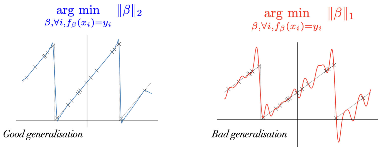
Better L1 or L2?

• \(f=\) linear regression with feature map: \(f(x)=<\beta,\phi(x)>\) \[\phi(x) = (\frac 1 k \cos(2\pi kx), \frac 1 k \sin(2\pi kx))_{k\leq d/2}\]

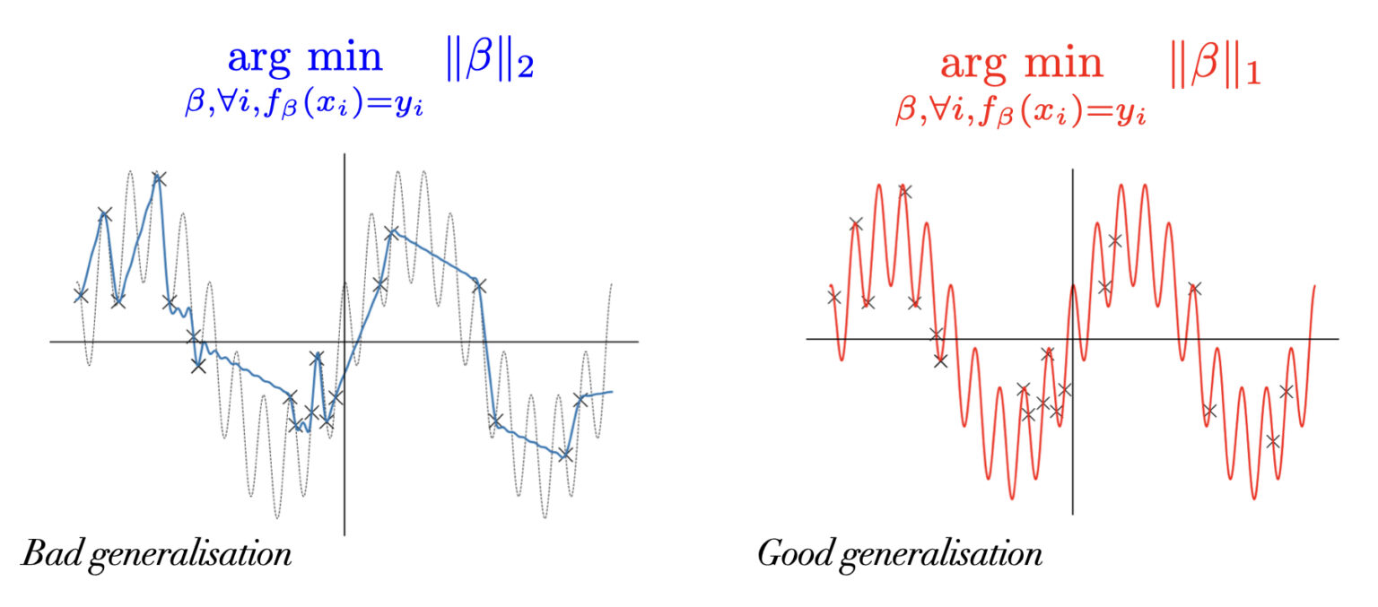
Better L1 or L2?

SGD vs. GD

Why does SGD work so well?

• Hyp 2: “flatness” of the local minimum found by SGD, which is related to the eigenvalues of the Hessian
  • Zhou paper studies SGD as a stoch. diff. equation
  • Show that the noise in SGD enables to more easily escape basin of attractions than Adam
  • see Bengio’s paper
  • high values of the ratio of learning rate to batch size leads to wider minima
  • cf. chapter 6 of this course

Why does SGD work so well?

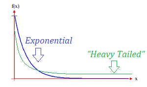
• Hyp 3: “heavy-tail” of the network weights at convergence

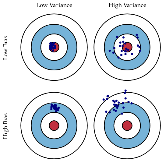
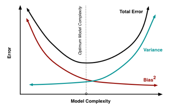
Bias-variance tradeoff

Depends on both classifier + learning method

• Let \(Z\) be a random variable with distrib \(P\)

• Let \(\bar{Z} = E_P[Z]\) be the average value of \(Z\)

Lemma: \[E\left[ (Z-\bar{Z})^2 \right] = E[Z^2] - \bar{Z}^2\]

• Let \(f\) be a real function, and our task be \(p(y|x)\) s.t. \(y=f(x)+\epsilon\)
  • with \(\epsilon \sim N(0;\sigma^2)\)

• We fit an hypothesis \(h(x) = w\cdot x +b\) with MSE over a training corpus

• Let be a new data point \(y = f(x) + \epsilon\):
  • What is the expected error ? \[E\left[ (y-h(x))^2 \right]\]

Expected over the training corpora of \(h\): \(x\) is constant

\(E[(h(x)-y)^2] = E[h^2(x)] -2E[h(x)]E[y] + E[y^2]\)

Apply the previous lemma to both square terms:

\(E[(h(x)-\bar{h(x)})^2] + \bar{h(x)}^2 -2\bar{h(x)}f(x) + E[(y-f(x))^2] + f(x)^2\)

Factorize:

\(E[(h(x)-\bar{h(x)})^2] + (\bar{h(x)} - f(x))^2 + E[(y-f(x))^2]\)

• (Wrong) intuition: it’s more important to reduce bias
  • Yes, on the average in the long run, low-bias models may perform well
  • But long run avgs are irrelevant in practice !
• Bagging helps to reduce variance:
  • resample corpus \(\rightarrow\) train multiple models
  • average predictions
  • Ex: Random forests

• Large bias: underfitting
  • Increase nb of parameters
• Large variance: overfitting
  • More regularization

Under/over-fitting

• Model “capacity” depends on nb of parameters + topology

How to find this optimum ?

• There are theoretical measures (see Aikake’s Information Criteria)
• But much better to use a development corpus

Overfitting in practice

• Fixed model capacity
• Never stop at “Nice, it’s compiling and running, I’m done!”:
  • Try to overfit on 1 batch, 10, 100…
  • Play with regularization
  • Find the broad “overfitting threshold”
  • What if I double the capacity?
  • …
• Art: interpreting the train and dev loss curves

Experiment, analyze, experiment, analyze…

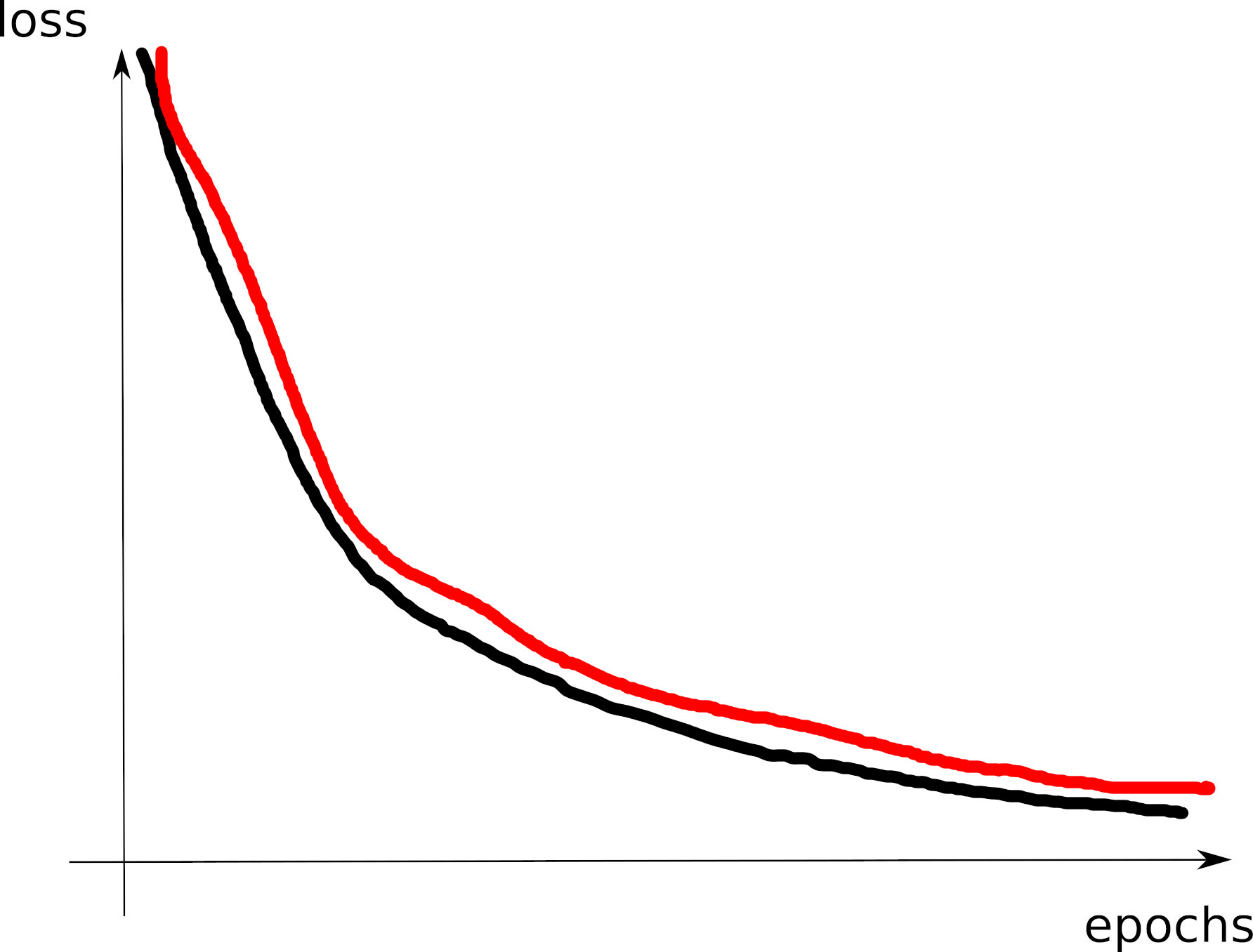
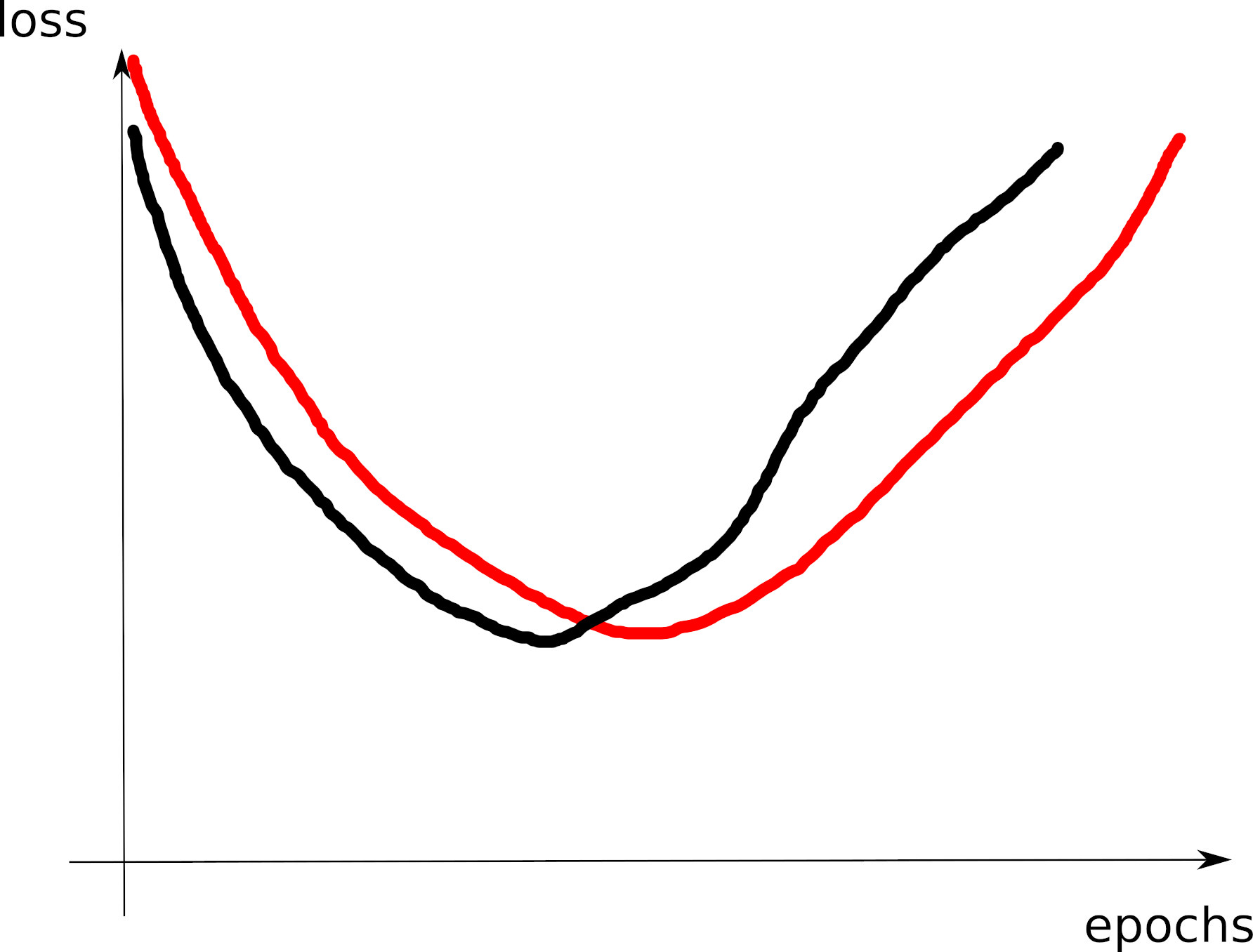
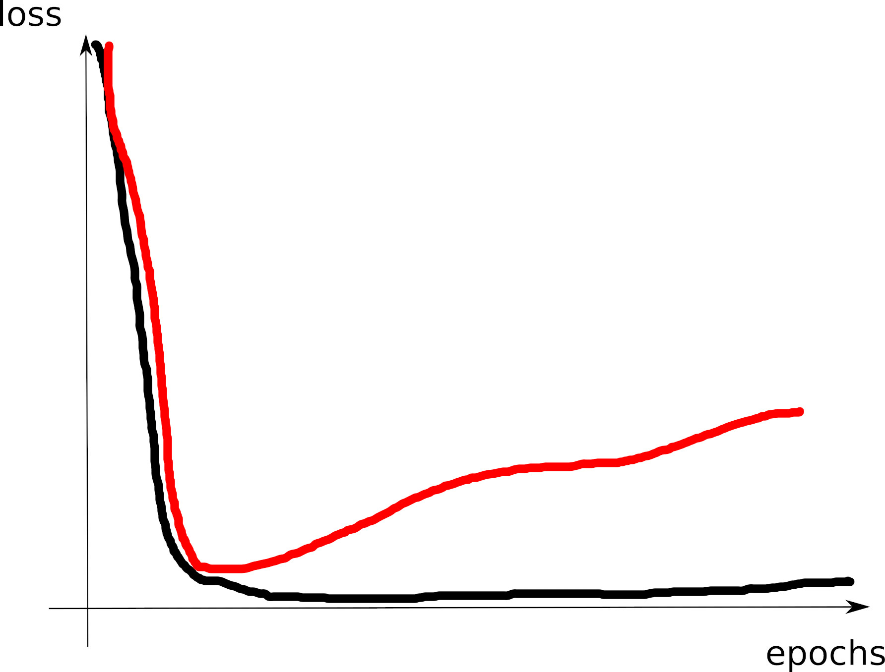
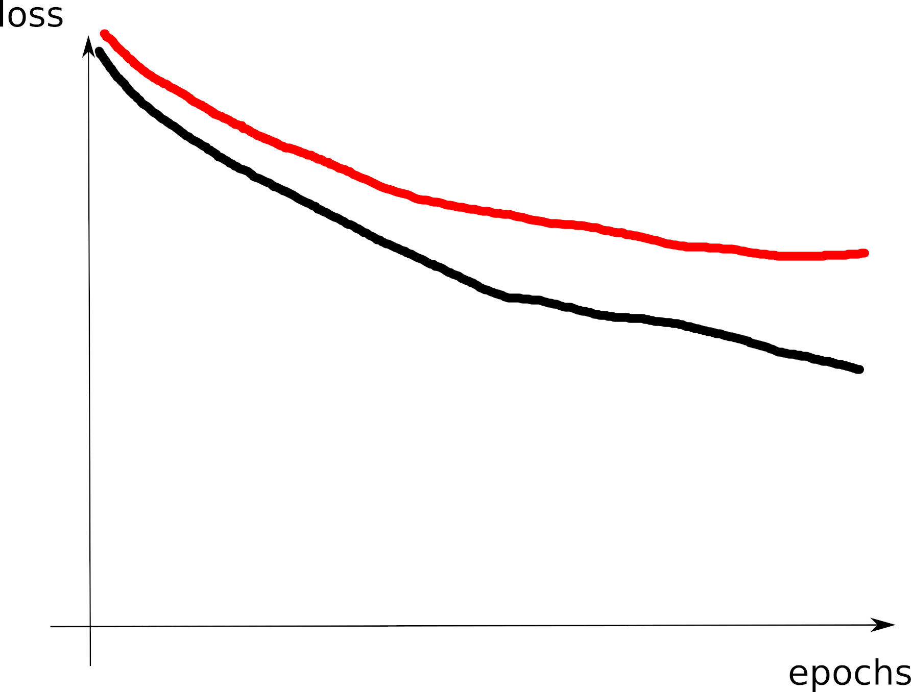
Train/dev loss curves

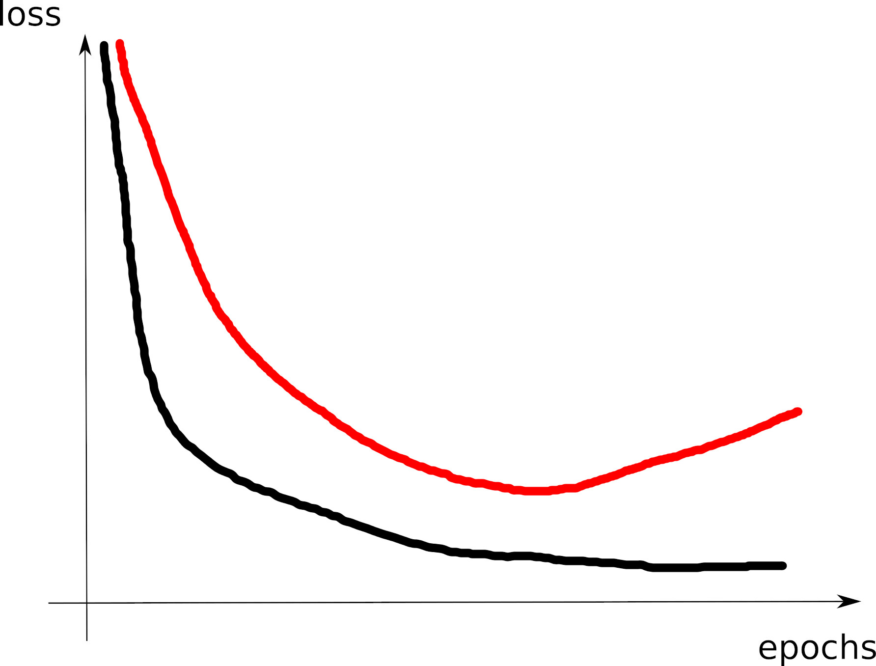
• C1: good curve: model around the overfitting threshold

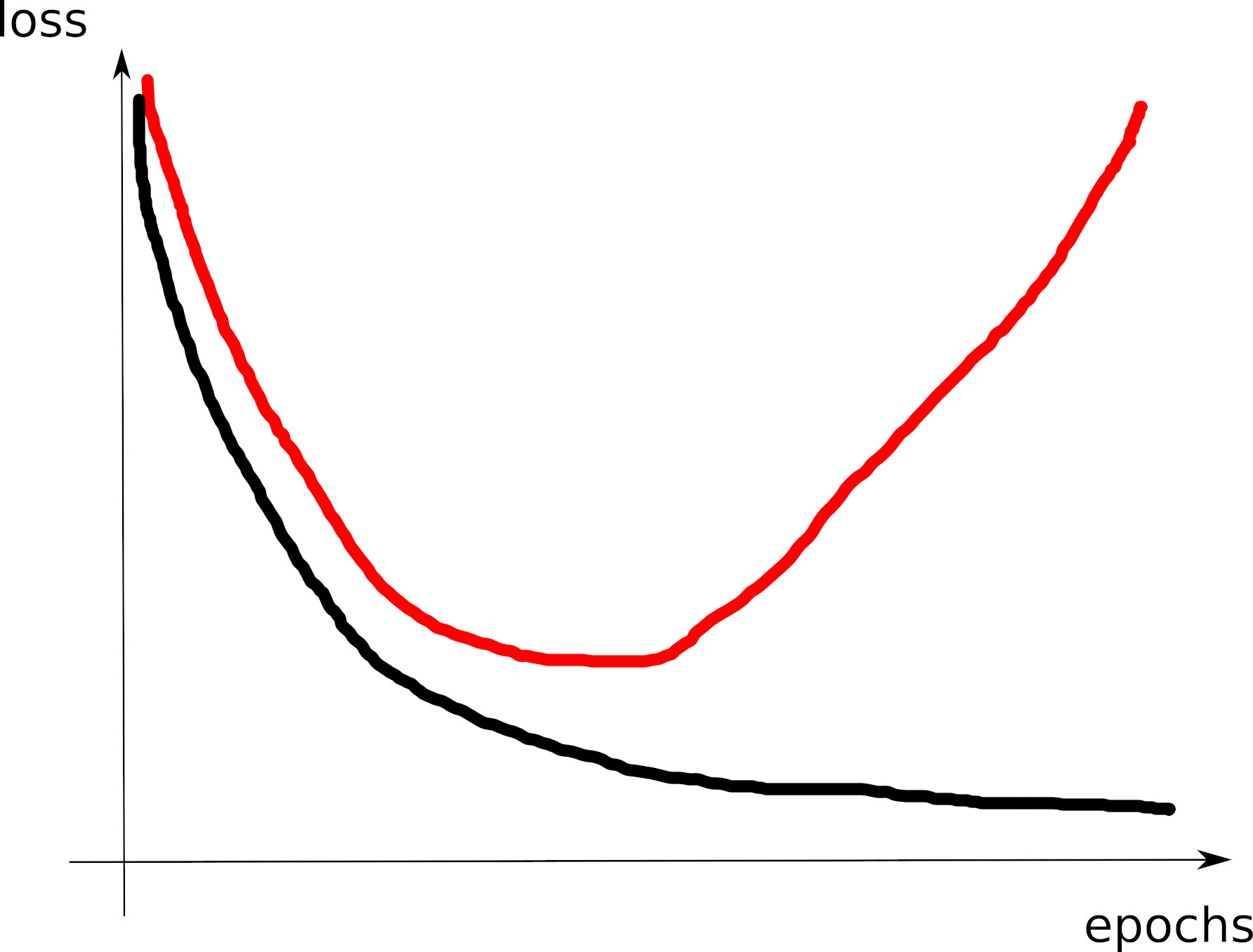
• C2: model (too far?) on the right of the overfitting threshold

• C3: model (too far!) on the left of the overfitting threshold

• C4: convergence issue: check LR

• C5: training loss=0: model capacity large (too large?)

• C6: large training loss: model capacity too small

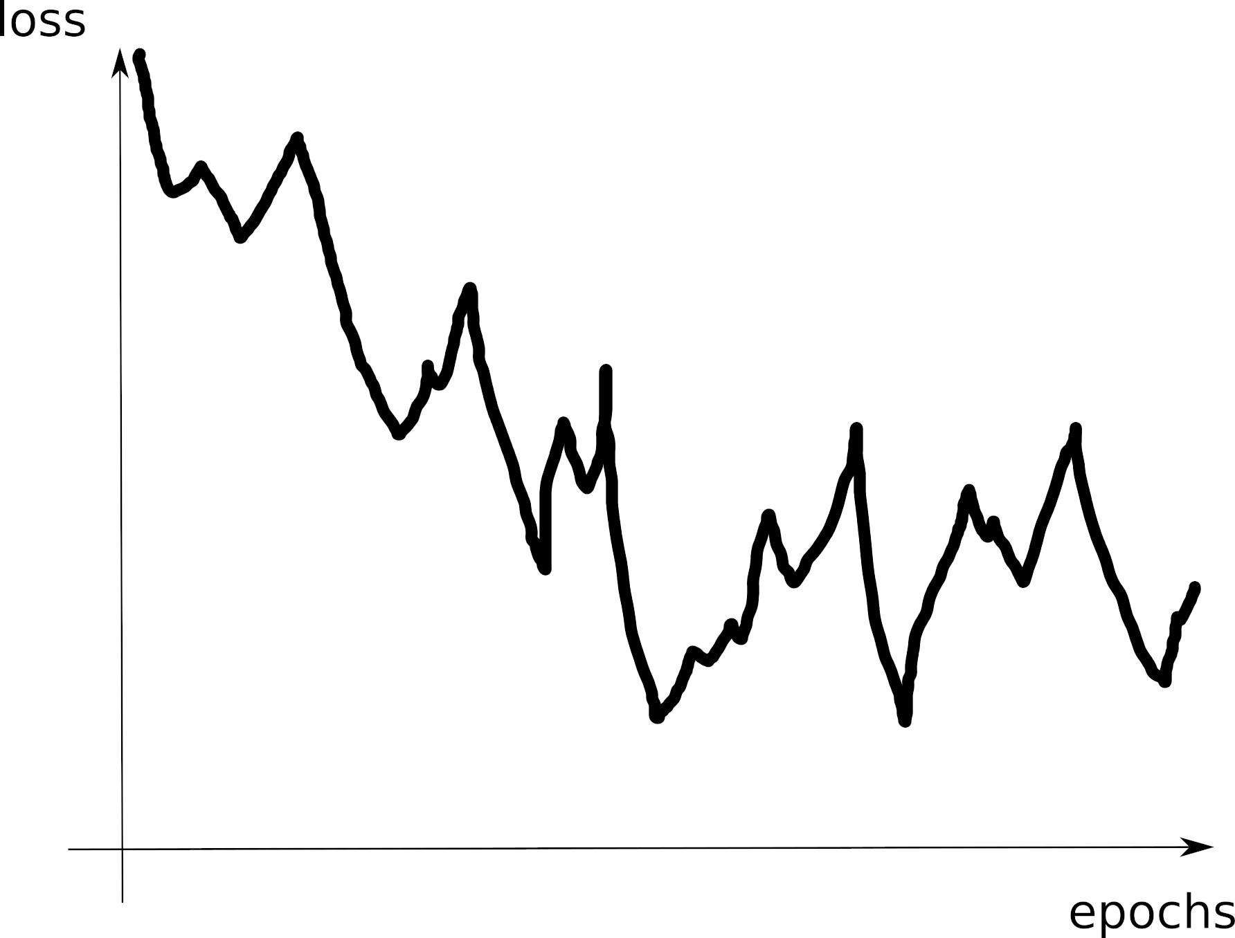
• C7: unstable training loss: reduce LR?

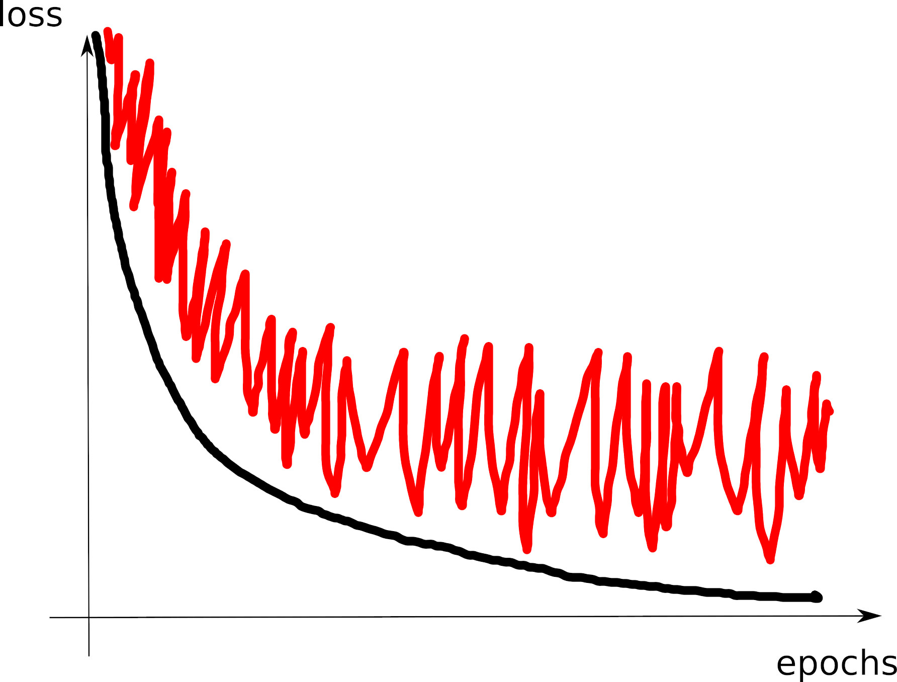
• C8: unstable dev loss: did you average it over the corpus?

Computing the loss

• Can be averaged over the whole corpus:
  • dev corpus usually small ==> OK
  • train corpus huge! LLMs are often trained over a single epoch
• Can be averaged over a batch
  • “just report every loss computed”
  • the smaller the batch, the larger the variability
  • running average since the beginning of the corpus?
• Can be averaged over \(n\) batches
  • much smoother curves, easier to interpret
  • but which value of \(n\)?

Train vs. Dev absolute loss values

• Are the train and dev loss values comparable?
• Sometimes, yes, often no:
  • “train” vs. “eval” mode: dropout…
  • should be representative of the distribution = averaged over enough data

Dev loss or accuracy curve?

• cross-entropy is strongly related to accuracy, but is different
• The loss can decrease either because:
  • the nb of errors decrease
  • the model becomes “over-confident” in its predictions

Overfitting is not bad-1

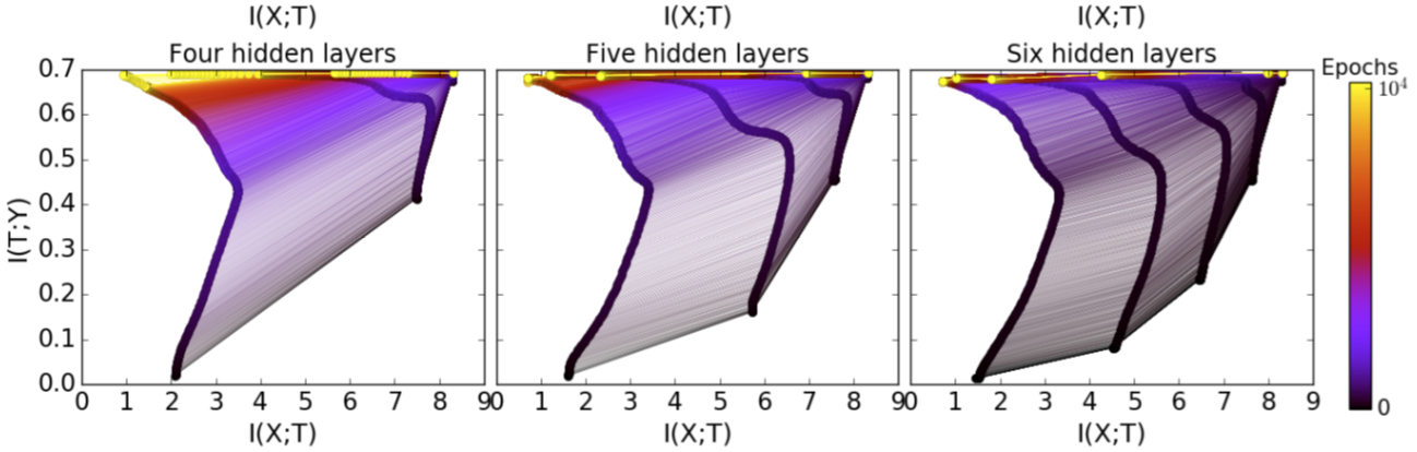
• Tishby’s “information bottleneck”

Tishby’s bottleneck

(Tishby, 2015)
https://arxiv.org/abs/1503.02406

• 2 phases: overtraining, then compression

Overfitting is not bad-2

• “double descent” (Belkin at al., arxiv 1812.11118, 2018)

Let us consider the following regression problem:

• gold (unknown) function \(f(x)=4(x-\frac 5 2)^2\)
• observations: 6 samples
  • (0,25) (1,9) (2,1) (3,1) (4,9) (5,25)

Inspired by https://mlu-explain.github.io/double-descent2/

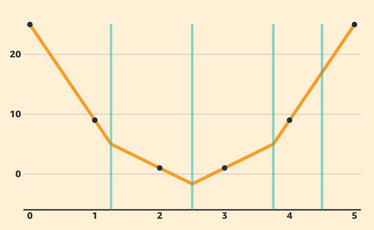
• model = piecewise linear fonction with fixed “knot points” \(t_k\):

\(g(x) = \alpha + \beta x + \sum_{k=1}^K \gamma_k \phi_k(x)\)

with

\(\phi_k(x) = \frac 1 2 |x-t_k|\)

• parameters = \((\alpha,\beta,\gamma_k)\)
• you can show \(g(x)\) is a parametrization of piecewise linear functions
  • the slope between two knots is constant = weighted sum of \(\gamma_k\)
  • you can make it equal to any piecewise linear = \(K\) linear eqs with \(K\) unknowns

• case \(K=0\): linear regression
• Implementation in pytorch: model:

class Knots(nn.Module):

    def __init__(self):
        super(Knots, self).__init__()
        self.alpha = nn.Parameter(torch.Tensor([0.]))
        self.beta  = nn.Parameter(torch.Tensor([0.]))

    def forward(self, X):
        return self.alpha + self.beta * X

• data:

traind = torch.utils.data.TensorDataset(
        torch.Tensor([0,1,2,3,4,5])/10.,
        torch.Tensor([25,9,1,1,9,25])/100.)
train_loader = torch.utils.data.DataLoader(traind, batch_size=6, shuffle=True)

• training loop:

def learn():
    nepochs = 50000
    lossf = nn.MSELoss()
    mod = Knots()
    opt = torch.optim.Adam(mod.parameters(), lr=0.01)
    for ep in range(nepochs):
        n,totloss = 0,0.
        for x,y in train_loader:
            n+=1
            opt.zero_grad()
            haty = mod(x)
            loss = lossf(haty,y)
            totloss += loss.item()
            loss.backward()
            opt.step()
        totloss /= float(n)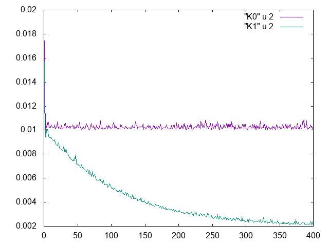
        print("TRAINLOSS",totloss,mod.alpha.item(),mod.beta.item())

• Exercice: plot the loss curve with \(K=0\)
• You should obtain:
  • horizontal line
  • loss plateaus at 0.11
  • underparametrized regime
  • model underfits

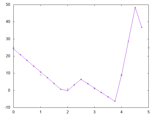
• With \(K=1\), you get (see exercice):

• At the interpolation threshold: solution determined by the knots:

• single choice per knot positions

• Let’s compute the expected error, when sampling the first knot uniformely between 1 and 2
• Let’s assume the first knot is at t0: \(P(t_0 \in [2-\epsilon; 2-\epsilon/2]) \propto \epsilon\)
• assume \(\epsilon<0.9\), then the knot is at best \((2-\epsilon,0.9)\) and the slope \(\geq 0.1/\epsilon\)
• so the error (q-norm) is at least in the order of \((1/\epsilon)^q\)

• Let’s consider the population of samples \((\epsilon = 1/2^m)_m\), each with probability \(\propto \epsilon\)
• The expected error is greater than the sum of the errors:

\[E[||\hat f - f||_q] \geq \sum_m^{\infty} \frac 1 {2^m} (2^m)^q = \sum_m^{\infty} 2^{m(q-1)}\]

• The error is infinite !

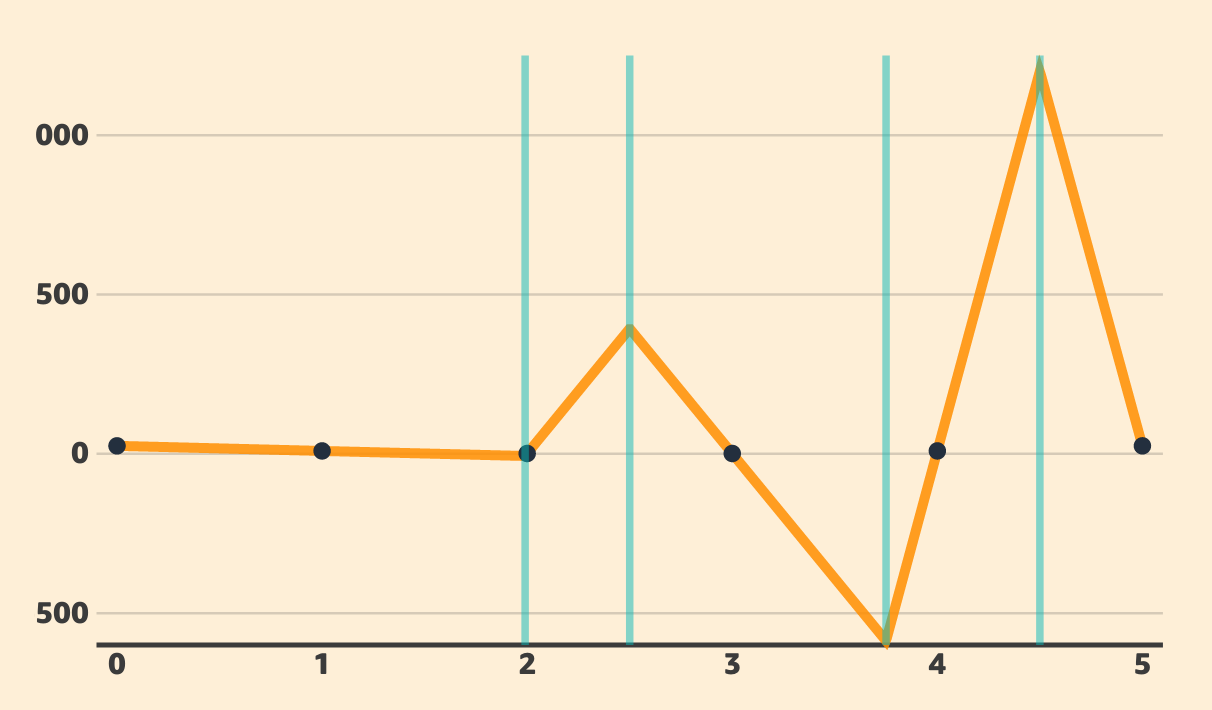
• loss curve at \(K=4\):

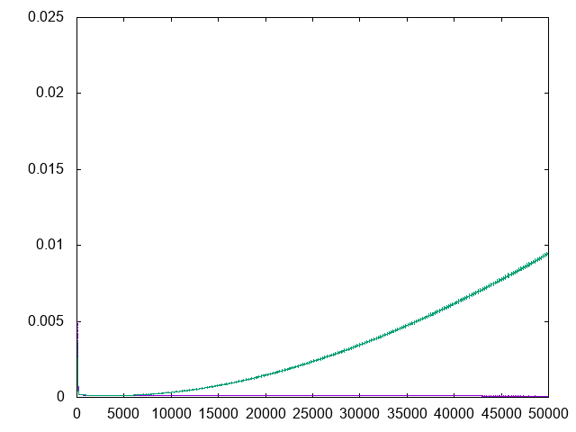
• Over-parametrized model:
  • more than one possible solution
• Let \(\delta_i\) be the slope of segment \(i\)
• \(\delta_{i+1}-\delta_i = \gamma_i\)
  • as when crossing \(t_i\), a single weight changes its sign in the sum of slopes \(g(x) = \alpha + \beta x + \sum_{k=1}^K \gamma_k \phi_k(x)\)

• Let \(\Delta_i\) be the distance btw the center of both segments
• Let’s assume we have many knots, so \(\frac {\delta_{i+1}-\delta_i}{\Delta_i} = \frac {\gamma_i} {\Delta_i}\) approximates the second derivative \(g''(t_i)\)

• Let \(p(x)\) be the uniform proba to sample \(t_i\)
• The proba that \(t_i\) lies in \(\Delta_i\) is approx. \(\Delta_i p(t_i)\)
• Alternative view: we know one of the \(K\) knots is there, so the proba it’s \(t_i\) is \(1/K\) \[\Delta_i \simeq \frac 1 {Kp(t_i)}\]

• So let us regularize our MSE loss by minimizing \(||\gamma||^2\):

\[||\gamma||^2 = \sum_k^K \gamma_k^2 \simeq \sum_k^K g''(t_k)^2 \Delta_k^2 \simeq \frac 1 K \sum_k^K \frac {g''(t_k)^2}{p(t_k)} \Delta_k\]

• This is an approx. of the integral of \(\frac {g''(t_k)^2}{p(t_k)}\)

\[||\gamma||^2 \simeq \frac 1 K \int \frac {g''(x)^2}{p(x)}dx\]

• assume \(p(x)\) is uniform on the domain, and \(g''(x)=0\) outside the domain, then we minimize \(\int_a^b g''(x)^2 dx\)
• so we look for an interpolation that is as close to linear as possible
• == natural cubic spline

• Extension to Multi-Layer Perceptron: proof by Singh & al., ICLR’22
• assumptions:
• MLP \(f()\) trained on data \(S\sim D\) to minimum \(\theta^*\)
• Empirical loss \(L_S\)
• covariance of loss gradients: \(C_L^{D} (\theta) = E_{z\sim D} [\nabla_{\theta} l(z,\theta) \nabla_{\theta} l(z,\theta)^T]\)
• covariance of function Jacobians: \(C_f^{S} (\theta) = \frac 1 {|S|} Z_S(\theta) Z_S(\theta)^T\)
• with \(Z_S(\theta)=[\nabla_{\theta} f_{\theta}(x_1), \dots, \nabla_{\theta} f_{\theta}(x_{|S|})]^T\)

• \(H_L^S(\theta^*)\) = Hessian of \(L\) estimated on the training corpus \(S\)
• \(r\) = rank of Hessian;
• \(\lambda_1,\dots,\lambda_r\) = eigenvalues of Hessian in decreasing order
• \(\lambda_{min}(A)\) = smallest eigenvalue of matrix \(A\);

• \(\sigma^2_{(x,y)} = ||\nabla_f l(f_{\theta^*}(x),y)||^2\)
• \(\exists\) a sample \((x,y) \sim D\) s.t. \(\sigma^2_{(x,y)>0}\)
• \(\alpha\) is the probability of \((x,y)\) in D;
• \(\tilde D = \{(x,y) \sim D : \sigma^2_{(x,y)}>0\}\);
• \(\sigma^2_{min} = \min_{(x,y)\sim \tilde D} \sigma^2_{(x,y)}\)

\(L(\theta^*) \geq \tilde {L_S}(\theta^*) + \frac 1 {n+1} \frac {\sigma_{min}^2 \alpha \lambda_{min} \left( C_f^{\tilde D} (\theta^*) \right)} {\lambda_r \left( H_L^S(\theta^*) \right) }\)

• with the “one-sample training loss” \(\tilde {L_S}(\theta^*) = E_{z\sim D}[l(z,\theta^*_{S\cup \{z\}})]\)
• What is important = \(\frac 1 {\lambda_r\left( H_L^S(\theta^*) \right)}\)

• Assume MSE Loss (and a few other hypothesis…):

\(L(\theta^*) \geq \tilde {L_S}(\theta^*) + \frac {\sigma_{min}^2 \alpha A \lambda_{min} \left( C_f^{\tilde D} (\theta^0) \right)} {B ||C_f^{D} (\theta^0)||_2 \left( \sqrt n - c \sqrt p \right)^2 }\)

• \(A\), \(B\) and \(c\) are constant
• \(\theta^0\) is initial model
• \(n\)=samples \(p\)=parameters
• Infinite for \(p=\frac 1 {\sqrt c}n\)

Grokking

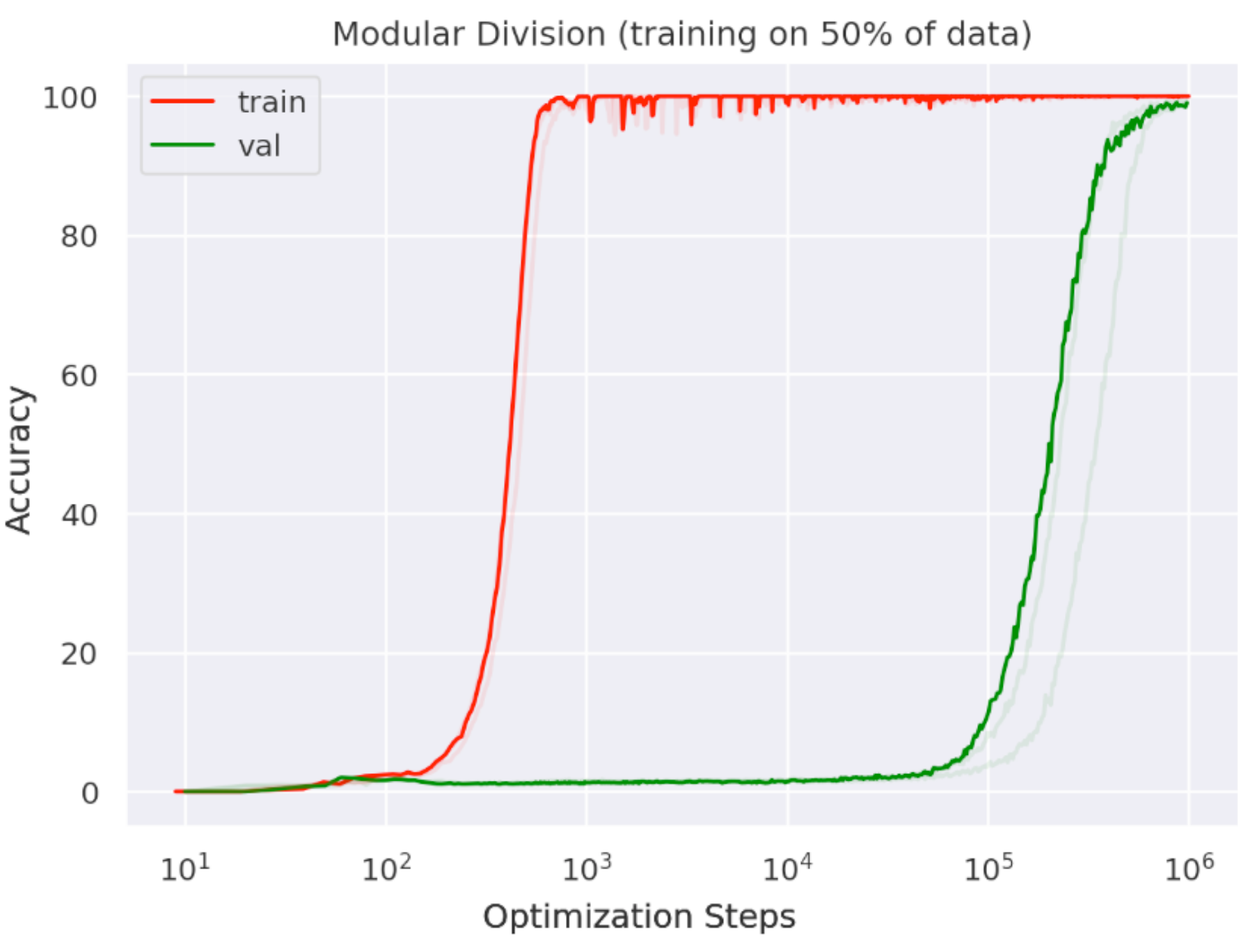
• First observed by Google in Jan 2022
  • Trained on arithmetic tasks
  • Must wait well past the point of overfitting to generalize
• It often occurs “at the onset of Slingshots” Apple paper
  • Slingshots = type of weak regularization = when “numerical underflow errors in calculating training losses create anomalous gradients which adaptive gradient optimizers like Adam propagate” blog
  • post-grokking solutions = flatter minima

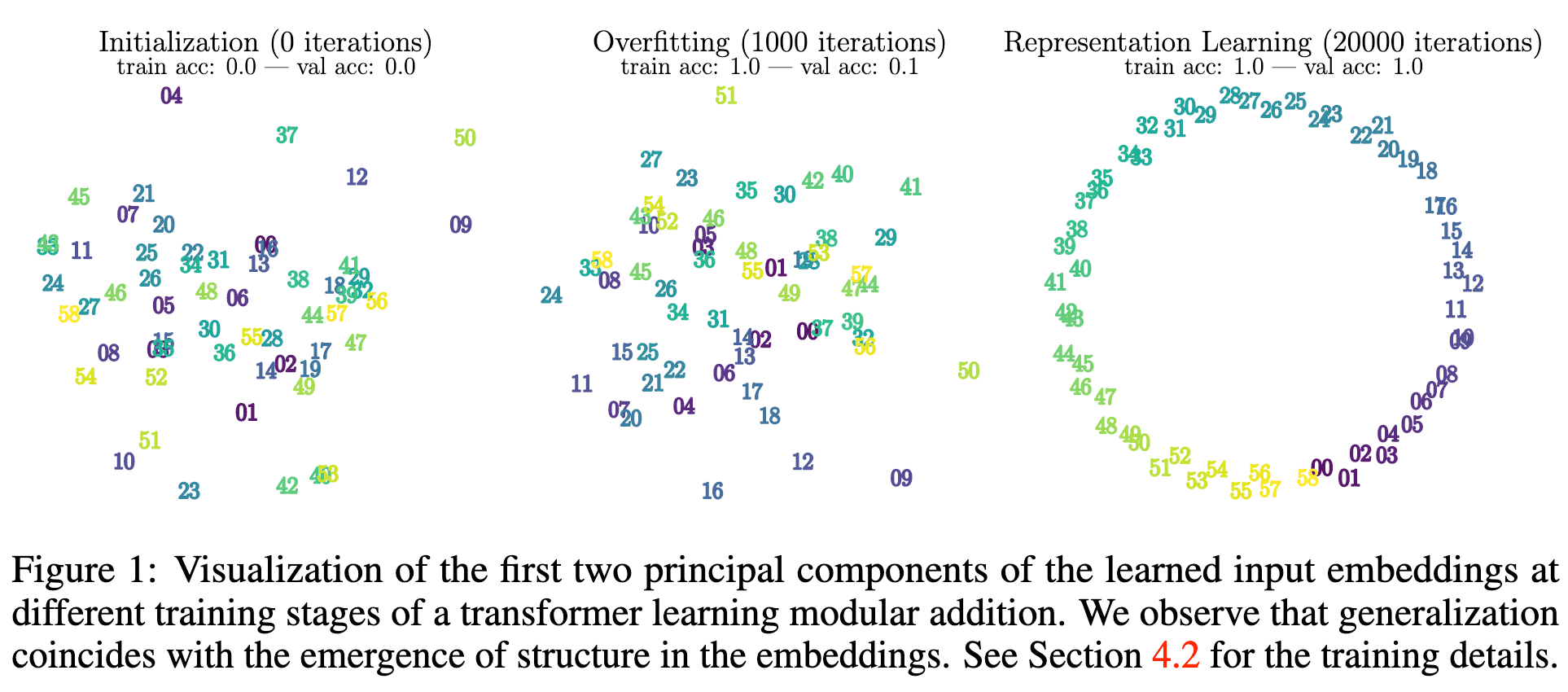
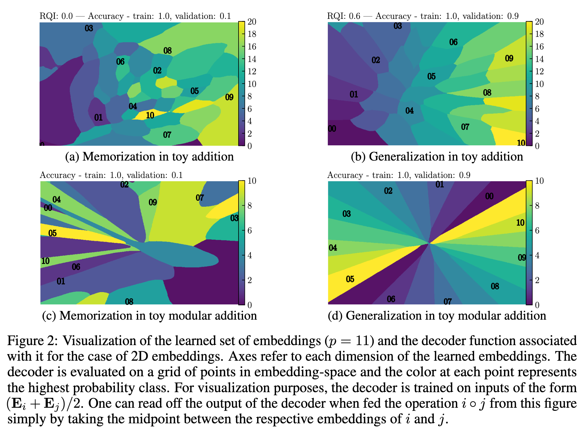
• Training involves multiple phase: grokking is one of them MIT paper
  • generalization, grokking, memorization and confusion
• When representations becomes structured, then generalization occurs:

• The 4 phases depend on hyper-parameters:

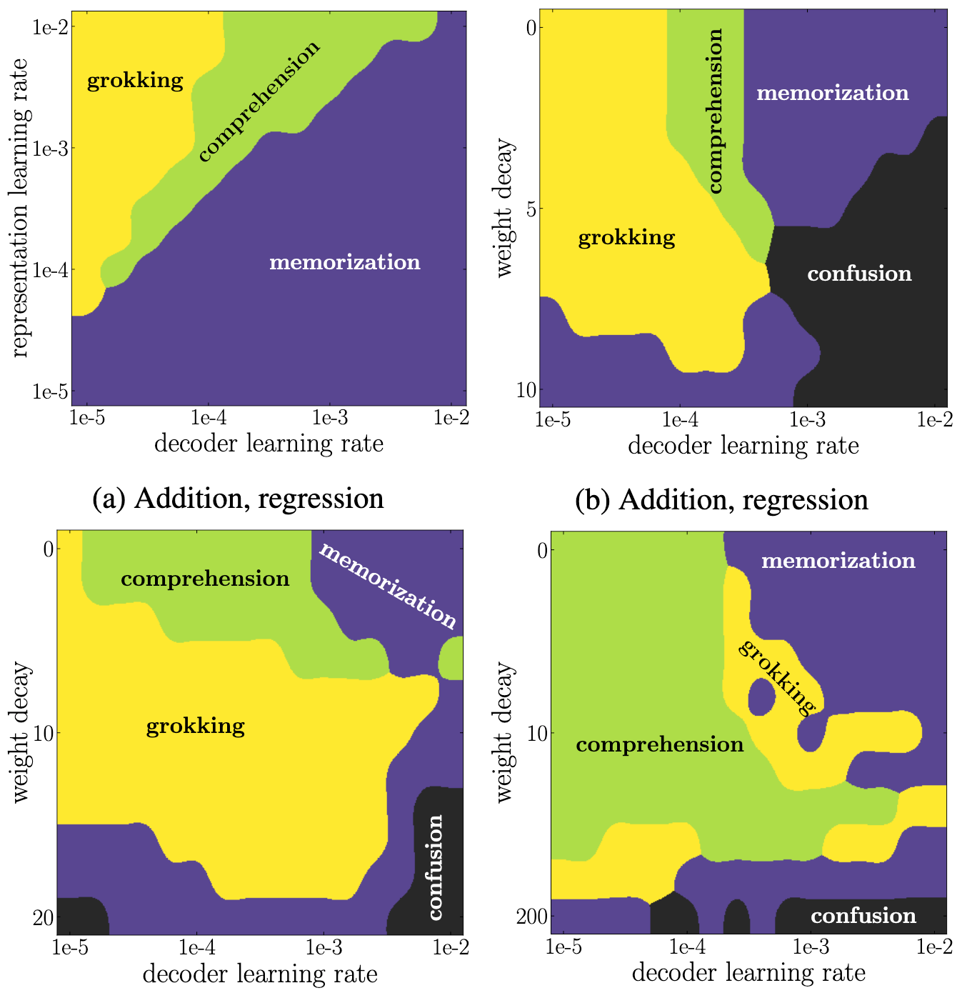
• Why do we observe phase during training?
  • NYU paper 2023
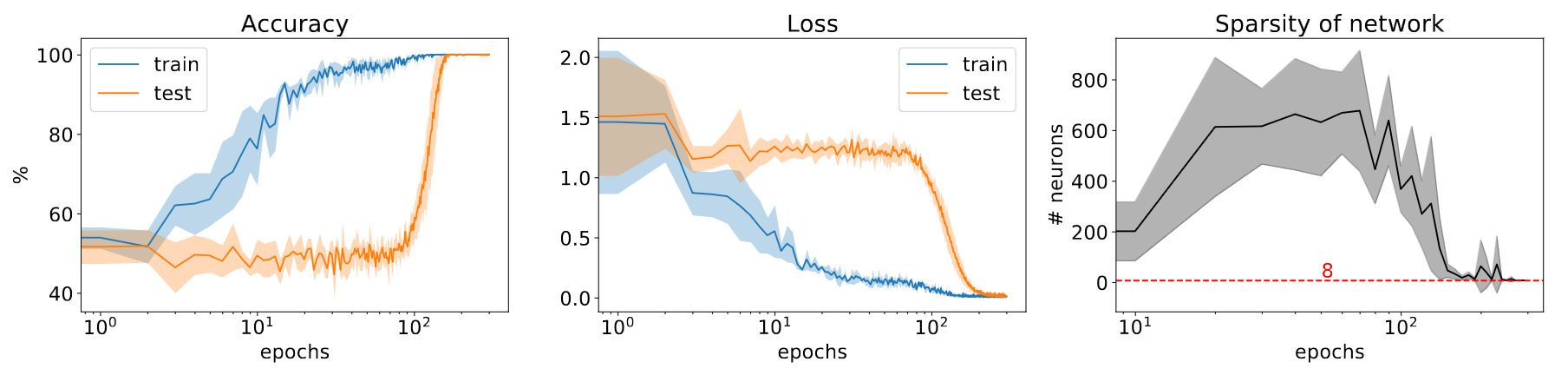
  • Because of competing sub-networks: dense for memorization and another sparse for generalization

• You have seen:
  • template code for pytorch
  • deep learning as differentiable programming
  • XPs for underfitting, interpolation point, over-parameterized
  • importance of regularization
  • double descent: why and when; grokking

• To be done in groups of 2 (or 1 student)
• Must give me by email a github link (or zip file with full GIT history, including .git/ dir) that contains:
  • A report in markdown or pure text format, with links to figures/curves
  • A code in python + pytorch
• deadline = 15 Decembre 2023

• Work to be done:
  • Choose a public dataset that you can train a deep learning model on
  • Create 1+ model(s) in pytorch that is based on/a combination of MLP, LSTM, ConvNet, Transformer
    • It’s OK to get inspiration from some code on the web, but you shall not just reuse one, and you must state in your report where you got inspiration from
  • Train it, evaluate, analyze and if possible iterate this process a few times

• Criteria used for grades:
  • Quality and depth of your analysis
  • Balanced contribution in the group (through GIT history)
  • Work progress over time (through GIT history)
• The report is by far the most important!
  • between 5 and 15 “pages”

• Download Meteo data
• Goal = predict the next T° given a seq of T°
• train on 2019, test on 2020
• Objectives:
  • template code for RNN & time series
  • use of Dataset & DataLoader
  • explore underfitting/overfitting
  • understand sources of variability

• Data: convert to tensor, then to Dataset, then to DataLoader:

# trainx = 1, seqlen, 1
# trainy = 1, seqlen, 1
trainds = torch.utils.data.TensorDataset(trainx, trainy)
trainloader = torch.utils.data.DataLoader(trainds, batch_size=1, shuffle=False)
testds = torch.utils.data.TensorDataset(testx, testy)
testloader = torch.utils.data.DataLoader(testds, batch_size=1, shuffle=False)
crit = nn.MSELoss()

• Model: simple RNN with a linear regression layer:

class Mod(nn.Module):
    def __init__(self,nhid):
        super(Mod, self).__init__()
        self.rnn = nn.RNN(1,nhid)
        self.mlp = nn.Linear(nhid,1)

    def forward(self,x):
        # x = B, T, d
        ...

• Every day, the RNN predicts the next day T°:
  • \(X\) is a tensor (Batch, Time, Dim) = (1, 365, 1)
  • \(\hat y_t = f(x_t)\)
  • loss: \(||\hat y_t - x_{t+1}||^2\)
  • all 365 predictions shall be processed in a single pass !
    • Look at both outputs of RNN in pytorch.org/docs

• compute MSE on test:

def test(mod):
    mod.train(False)
    totloss, nbatch = 0., 0
    for data in testloader:
        inputs, goldy = data
        haty = mod(inputs)
        loss = crit(haty,goldy)
        totloss += loss.item()
        nbatch += 1
    totloss /= float(nbatch)
    mod.train(True)
    return totloss

• Training loop:

def train(mod):
    optim = torch.optim.Adam(mod.parameters(), lr=0.001)
    for epoch in range(nepochs):
        testloss = test(mod)
        totloss, nbatch = 0., 0
        for data in trainloader:
            inputs, goldy = data
            optim.zero_grad()
            haty = mod(inputs)
            loss = crit(haty,goldy)
            totloss += loss.item()
            nbatch += 1
            loss.backward()
            optim.step()
        totloss /= float(nbatch)
        print("err",totloss,testloss)
    print("fin",totloss,testloss,file=sys.stderr)

• The Main:

mod=Mod(h)
print("nparms",sum(p.numel() for p in mod.parameters() if p.requires_grad),file=sys.stderr)
train(mod)

• Step 1: copy/paste + complete this code and run a training
  • check convergence!
• Step 2: compare and analyze \(h=1\), \(h=100\)
• Step 3: rerun multiple times: what’s the variability and why?

• Underfitting regime:
  • Take the “knots” code with \(K=0\) in the course and modify it to add 1 parameter \(K=1\)
  • Plot the loss curve and try to obtain a similar one as in the course

• Overfitting regime:
  • modify the code with \(K=4\)
  • generate a test set composed of 20 uniform samples and plot both the train and test loss
  • try to get curves that clearly overfit

Book: deep learning with pytorch

• Exercice from B. Favre

• Avec l’aide de la documentation pytorch, calculez l’expression suivante: \[a = 1_{(3 \times 2)}\] \[b = \sin(1+\sqrt{3I_2} + 5 ||a||)\]

Exercice: combine CNN and RNN

• you have a “long” time series with 3000 timesteps. You want to handle it by using first a CNN with kernel=3 and stride=3 that will reduce it to 1000 timesteps, and then an LSTM.
• The goal is to classify the full sequence into N classes (e.g., whether the sequence of temperature has been recorded in winter or summer…)
• write both methods of the model: init() and forward()