Machine Learning
& differentiable programming
Christophe Cerisara - 2023-2024
Introduction
Prerequisites
- Frédéric Sur’s course on Machine Learning
- (optional: Erwan Kerrien’s course on deep learning for image processing)
- Good knowledge of python3 and GIT
- Have pytorch installed and ready to use
Course content
- Focus on Deep Learning:
- Intro: DL and programming
- chapter 1: notations, reminders
- chapter 2: overfitting, double descent, grokking
- chapter 3: transformers, scaling laws, emergence
- chapter 4: best practices
- chapter 5: uncertainty modeling
- chapter 6: loss landscape geometry
Evaluation
MCQs in class (coef 1)
mini-project (coef 2)
send to cerisara@loria.fr
Mini-project
- (to be precised)
- you propose a project that:
- trains deep learning model on data
- evaluates the model
- You give:
- a source code with GIT history
- individual contributions to GIT history will be evaluated
- Report:
- the problem: where you get data from, what is done elsewhere
- your solution: where do you get your inspiration from, describe your approach, why you adopt it
- summarize experiments, evaluation, analyse the results
- concludes
A note on Jupyter
- Recommend to not use jupyter
- Good for educative purpose
- Bad for software engineering:
- not designed for GIT, CI, collaboration
- not designed for large or structured code
- not designed for grids, automatization
Other courses
Course material
Questions?
- course website: https://members.loria.fr/CCerisara/#courses/machine_learning/
- contact: cerisara@loria.fr
Intro: DL vs. ML
Machine Learning
- Given a model (SVM, Decision Tree, Bayesian Network…), how to train it?
- Goal:
- Find an algorithm for training the model
- Prove convergence
- Based on maths:
- proof, compute bounds
Deep Learning
- Given data, how to design a model (= program) to capture information
from data?
- Don’t care (much) about training algorithm, convergence
- Goal: design a model
- Based on programming:
- Which program may extract relevant information from this type of data?
- Deep Learning is not about stacking LSTM, CNN and MLP!
- DL is about designing a program
- DL is fundamentally empirical
- Any (maths) theory? Yes, but embryonic!
- What happens during training? (emergence, grokking, dble descent…)
- Geometric properties of the loss manifold
- How does it scale?
- How is information stored? reasoning appears?…
Intro: links btw programming and Deep Learning
- DL is based on differentiable programming
- LLMs can learn how to program
- LLMs use programs to reason
- LLMs accompagny evolution of programming
- LLMs will replace developers?
DL = differentiable programming
“Deep” model
def f(x):
  if x>C: x*=2
  else:   x*=3
  return x
Training
data= (3,10)
err = (f(3)-10)**2
err.backward()  # calc dérivée
C -= 0.1*C.grad # diminue erreur
LLMs can learn how to program
- LLMs take a text in, and generate its continuation: “How can I draw a sinusoid in javascript?”
To draw a sinusoid in JavaScript, you can use the Canvas API. Here's an example of how to do it:

// Get the canvas element
var canvas = document.getElementById("myCanvas");
var ctx = canvas.getContext("2d");

// Define the sinusoid parameters
var amplitude = 100;
var frequency = 1;
var phase = 0;
var x = 0;

// Draw the sinusoid
for (var i = 0; i < canvas.width; i++) {
 var y = amplitude * Math.sin(frequency * i + phase);
 ctx.beginPath();
 ctx.moveTo(x, y);
 ctx.lineTo(x + 1, y);
 ctx.stroke();
 x++;
}

This code will draw a sinusoid with the specified amplitude, frequency, and phase, and will update the canvas as the user scrolls.
LLMs use programs to reason
“Train 1 departs at 6 AM from city A and arrive in city B in 11 AM. Train 2 departs at 7:30AM from city B and arrive in City A at 11 AM. When will both trains meet?”
train1_travel_time = 11 - 6
# 7:30 AM refers to 7.5
train2_travel_time = 11-7.5
dist_a_b = Symbol("D",positive=True)
train1_speed = dist_a_b / train1_travel_time
train2_speed = dist_a_b / train2_travel_time
ans = dist_a_b / (train1_speed + train2_speed)- LLM input = examples of search over a problem
- Ex: Game of 24:
Use numbers and basic arithmetic operations (+ - * /) to obtain 24. When considering the next steps, do not choose operations that will result in a negative or fractional number. In order to help with the calculations, the numbers in the parenthesis represent the numbers that are left after the operations and they are in descending order...

 User:
11 7 4 1
Assistant:
Let’s consider the most promising first steps:
1. 7 * 4: (28, 11, 1)
2. 7 + 1: (11, 8, 4)
3. 4 + 1: (11, 7, 5)
4. 11 - 4: (7, 3, 1)
Let’s consider the most promising second steps:
1. (28, 11, 1)
- 28 - 11: (17, 1)
- 28 - 1: (27, 11)
- 11 + 1: (29, 28)
- 11 - 1: (28, 10)
2. (11, 8, 4)
- 11 + 8: (19, 4)
- 8 + 4: (12, 11)
- 11 - 8: (4, 3)
- 8 - 4: (7, 11)
3. (11, 7, 5)
- 11 - 5: (7, 6)
- 7 - 5: (11, 2)
- 7 * 5: (35, 11)
- 11 + 5: (16, 7)
4. (7, 3, 1)
- 7 - 3: (4, 1)
- 7 * 3: (21, 1)
- 3 + 1: (7, 4)
- 7 - 1: (6, 3)
Let’s consider the most promising third steps:
1. 7 * 4 = 28
- 28 - 11: (17, 1): 18, 16, 17, 17
- 28 - 1: (27, 11): 38, 16, 297, 2.45
- 11 + 1: (29, 28): 57, 1, 812, 1.03
- 11 - 1: (28, 10): 38, 18, 280, 2.8
2. 7 + 1 = 8
- 11 + 8: (19, 4): 23, 15, 76, 4.75
- 8 + 4: (12, 11): 23, 7, 132, 3
- 11 - 8: (4, 3): 7, 1, 12, 1.33
- 8 - 4: (7, 11): 18, 4, 77, 1.75
3. 4 + 1 = 5
- 11 - 5: (7, 6): 13, 1, 42, 1.17
- 7 - 5: (11, 2): 13, 9, 22, 5.5
- 7 * 5: (35, 11): 46, 24 = 35 - 11 -> found it!
Backtracking the solution:
Step 1:
4 + 1 = 5
Step 2:
7 * 5 = 35
Step 3:
35 - 11 = 24
Considering these steps: 24 = 35 - 11 = (7 * 5) - 11 = (7 * (4 + 1)) - 11 = 24.
answer: (7 * (4 + 1)) - 11 = 24.
Evolution of programming?

LLMs will replace developers?
- No!
- LLMs are creative, but in a different way than humans
- LLMs lack affects, do not understand a situation as humans
- Only humans are accountable, and thus shall be in control
- …
Notations, reminders of basic notions
- A task is a distribution \(p(x,y)\)
- \(x \in \mathcal{X}=R^{T\times W\times H\times d\dots}\) are the observations
- \(y \in \mathcal{Y}\) are the
gold labels (ground truth)
- \(\mathcal{Y}=\) finite set, it’s a classification task
- \(\mathcal{Y}=\mathcal{X}\), it’s a regression task
- \(\mathcal{Y}=R^{T'\times V\dots}\), it’s a generation task: “generate a textual description of a video”
- detection task: \(\exists y_0\in \mathcal{Y} : p(y_0) >> p(y) ~~~ \forall y\neq y_0\)
- multi-label classification: \(y\) is a tuple
- sequential decision tasks: find trajectory in \(\mathcal{X}=\{seq~of~(states,actions)\}\) with \(\mathcal{Y}\) sparse
- …
Basic archi: for a classification task with \(N\) labels, you stack:
- Representation module: \(z=f_\theta(x)\) with \(z\in R^h\)
- followed by classification layer: \(y = W z\) with \(y\in R^N\)
- \(y\) are called the logits
- \(y\) can be normalized into class posterior probabilities with softmax
- decision rule: \(class = \arg\max_i y_i\)
Training:
- compute the loss:
- cross-entropy between posteriors and gold distribution
- equivalent to negative log-likelihood
- often, you don’t need to explicit the softmax: it’s integrated within the cross-entropy
Special output cases:
- binary classif:
- 2 neurons (with softmax) (X-ent)
- 1 neuron with sigmoid (binary X-ent)
- multi-label: N neurons with sigmoid (MSE)
- regression: same as input size, with linear (MSE)
- ranking, IBL…: 1 neuron=score with linear
Special input features:
- Symbols/discrete features: one-hot vector
- Varying-length sequences: truncating/padding
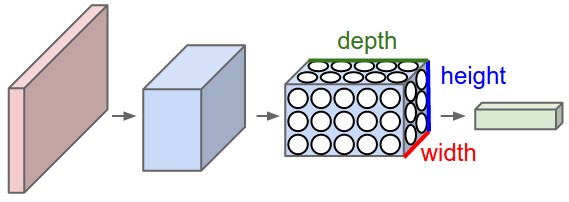
- dimensionality is often decomposed: \(\mathcal{X}=R^{T\times W\times H\times d}\), so \(x\) is represented by a tensor in deep learning toolkits
- a DL model \(f_{\theta}(x)\) is a “function” (program)
with parameters \(\theta\) that represents \(\hat p_{\theta}(x,y)\)
(generative model) or \(\hat
p_{\theta}(y|x)\) (discriminative model)
- generative: VAE, GAN, Flow, diffusion…
- discriminative: ResNet…
- Loss:
- We note \(\hat y\) the prediction of the model
- It may be different for each run: \(\hat y \sim \hat p_{\theta}(y|x)\)
- prediction error (or loss): \(l(\hat y, y)\) with \(l\) the loss function (hinge loss, MSE, cross-entropy…)
- Risk:
- classifier risk: \(R(\theta) = E_{p(x,y)}\left[ l(f_{\theta}(x),y) \right]\)
- a.k.a. population risk
- labeled corpus: \(\mathcal{D} = \left\{(x_i,y_i) \sim p(x,y)\right\}_{1\leq i\leq n}\)
- unlabeled corpus: \(\mathcal{U} = \left\{x_i \sim p(x) = \int p(x,y)dy\right\}_{1\leq i\leq n}\)
- empirical risk: \(R_e(\theta,\mathcal{D}) = E_{\mathcal{D}}\left[ l(f_{\theta}(x),y) \right]\)
- training objective: \(\hat \theta = \arg\min_{\theta} R(\theta)\)
- supervised training: \(\hat \theta = \arg\min_{\theta}
R_e(\theta,\mathcal{D})\)
- it is just an approximation of the true classifier risk, except in toy tasks: XOR…
- this approximation is the root cause of overfitting
- When you optimize \(R_e\) with SGD over a single epoch (i.e., only seeing new samples at every step), then SGD directly optimizes the true risk (see Francis Bach’s blog)
- … but you may still overfit with finite data!
- \(f_{\theta,\varphi}(x)\) has hyper-parameters \(\varphi\) that are not optimized on the training corpus: type of model, number of layers, training procedure…
- \(\varphi\) must be optimized on a development corpus
- the final model \(f_{\hat\theta,\hat\varphi}(x)\) must be evaluated on the test corpus only once: never evaluate again on the test corpus with another \(\hat\varphi'\)!!
- evaluation is very difficult and requires a lot of thinking:
- which important generalization properties should be evaluated? over image capturing devices? over photo conditions (night, rain…)? over time? over domains?…
- design an adequate test corpus
- end-to-end training: one model from the raw observations to the labels vs.
- cascade training: several model parts trained independently
- Entropy of a probability distribution = nb of bits required to encode the distribution \[H(p)=-\sum_i p_i \log p_i\]
- Cross-entropy between 2 distributions = nb of bits required to encode one distribution, when we only know another distribution \[H(p,q)=-\sum_i p_i \log q_i\]
- Kullback-Leibler divergence = \(H(p,q)-H(p)\) \[KL(p||q)= \sum_i p_i \log \frac {p_i}{q_i}\]
- Training goal: make a parametric distribution \(q\) fit a gold distribution \(p\)
- Equivalent to minimize KL or minimize X-ent
- Equivalent to minimize the negative log-likelihood
- a.k.a. maximize likelihood estimation (MLE)
Regularization
Naive DNN overfits \(\rightarrow\) we want to reduce variance
This can be done by adding a term to the loss that limits the space where parameters can live:
- L2 regularization is the most common: \[loss = E[H(p,q)] + \lambda \sum_i \theta_i^2\]
L2 Regularization
L2 can be interpreted as adding a Gaussian prior:
see p. 324 of Larry Bayesian Inference book
Assume simple linear model \(y=\beta x + \epsilon\)
- With noise \(\epsilon \sim N(0,\sigma^2)\)
- With one random parameter \(\beta\)
So cond. likelihood is \(p(y|x,\beta) = \prod_t N(y_t;\beta x_t,\sigma^2)\)
- Let’s apply a Gaussian prior on our parameter: \[\beta \sim N(0, \lambda^{-1})\]
- Combine likelihood and prior: \[p(y|x,\beta)p(\beta) = \prod_t N(y_t;\beta x,\sigma^2)N(\beta;0, \lambda^{-1})\]
- With log: \[\sum_t -\frac 1 {\sigma^2} (y_t - \beta x_t)^2 - \lambda \beta^2\]
- This is neg-log-like + L2
Other regularizations
- L1 \[loss = E[H(p,q)] + \lambda \sum_i |\theta_i|\]
- Dropout
- Randomly remove \(\lambda\)% input and hidden neurons
data augmentation: Replicate dataset by adding \(\lambda\)% noise
SGD: Tune mini-batch size
Weights initialization
Why initialization is important ?
- If the weights start too small, the signal shrinks as it pass through until it’s too tiny to be useful
- If the weights start too large, the signal grows as it pass through until it’s too large to be useful
So we want the variance of the inputs and outputs to be similar !
Xavier initialization
For each neuron with \(n_{in}\) inputs:
- Initialize its weights \(W\) from a zero-mean Gaussian with
\[Var(W)=\frac 1 {n_{in}}\]
Refs: http://andyljones.tumblr.com/post/110998971763/an-explanation-of-xavier-initialization
Glorot initialization
For each neuron with \(n_{in}\) inputs, going into \(n_{out}\) neurons:
- Initialize its weights \(W\) from a zero-mean Gaussian with
\[Var(W)=\frac 2 {n_{in} + n_{out}}\]
http://pytorch.org/docs/master/nn.html?highlight=torch nn init#torch.nn.init.xavier_normal
Batch normalization
- You must normalize your data; in addition, you may do:
- batch-norm: one neuron, normalize over batch
- layer-norm: one batch, normalize over neurons
- … so that the mean=0 and standard deviation=1
- May have parameters to further scale + shift
- Recommended readings:
- https://kratzert.github.io/2016/02/12/understanding-the-gradient-flow-through-the-batch-normalization-layer.html
- http://pytorch.org/docs/master/nn.html?highlight=batchnorm1d#torch.nn.BatchNorm1d
A lot of tricks
“simple” MLP?
- Find a good topology, residual connections, parameter sharing…
- Find a good SGD variant
- Tune learning rate, nb of neurons…
- Tune regularization strength, dropout…
- Laye + batch normalization
- Tune nb of epochs, batch size…
Andrew Ng: “If you tune only one thing, tune the learning rate!”
Practice: deep learning toolkits
- Why scikit-learn is not enough?
- autoGrad
- seamless cuda support
- predefined modules: conv, LSTM, X-ent…
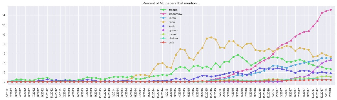
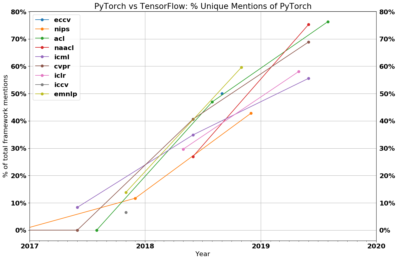
- Main research DL libs: pytorch, tensorflow, jax
- For embedded/industry: Caffe, MXNet, Torchscript, js…
- ONNX = Standard model format?
- These toolkits work as follows:
- python code \(\rightarrow\) computation graph G
- Iterate:
- data input into G \(\rightarrow\) outputs \(\hat y\) (forward)
- compute loss and \(\nabla_{\hat y} l(\hat y,y)\) at the output
- backpropagate in G (backward) to compute \(\nabla_{\theta} l(\hat y,y)\)
- gradient descent step: \(\theta \leftarrow \theta - \epsilon \nabla_{\theta} l(\hat y,y)\)
Autodiff
Autodiff = set of techniques to numerically evaluate the derivative of a function specified by a program
Exemple of computation graph:
- Forward pass: computes values from inputs to outputs (in green)
- Backward pass: recursively applies chain rule to compute gradients (in red) from the end to the inputs
Every gate in the circuit computes its local gradient with respect to its output value.
Backprop = local process
- Example: the “+” gate: \(x + y =
q\)
- It is equiped with local derivative:
- To its first input: \(\frac {dq}{dx}=1\)
- To its second input: \(\frac {dq}{dy}=1\)
- It is equiped with local derivative:
- Assume it is given a gradient value \(\frac {df}{dq}\) at its output:
- It passes it to its first input by multiplying it with its local derivative: \(\frac {df}{dq} \times \frac {dq}{dx} = \frac {df}{dx}\)
- It passes it to its second input by multiplying it with its local derivative: \(\frac {df}{dq} \times \frac {dq}{dy} = \frac {df}{dy}\)
- Don’t specialize in one specific tool/model
- Better understand the theoretical principles
- They’re evolving very fast
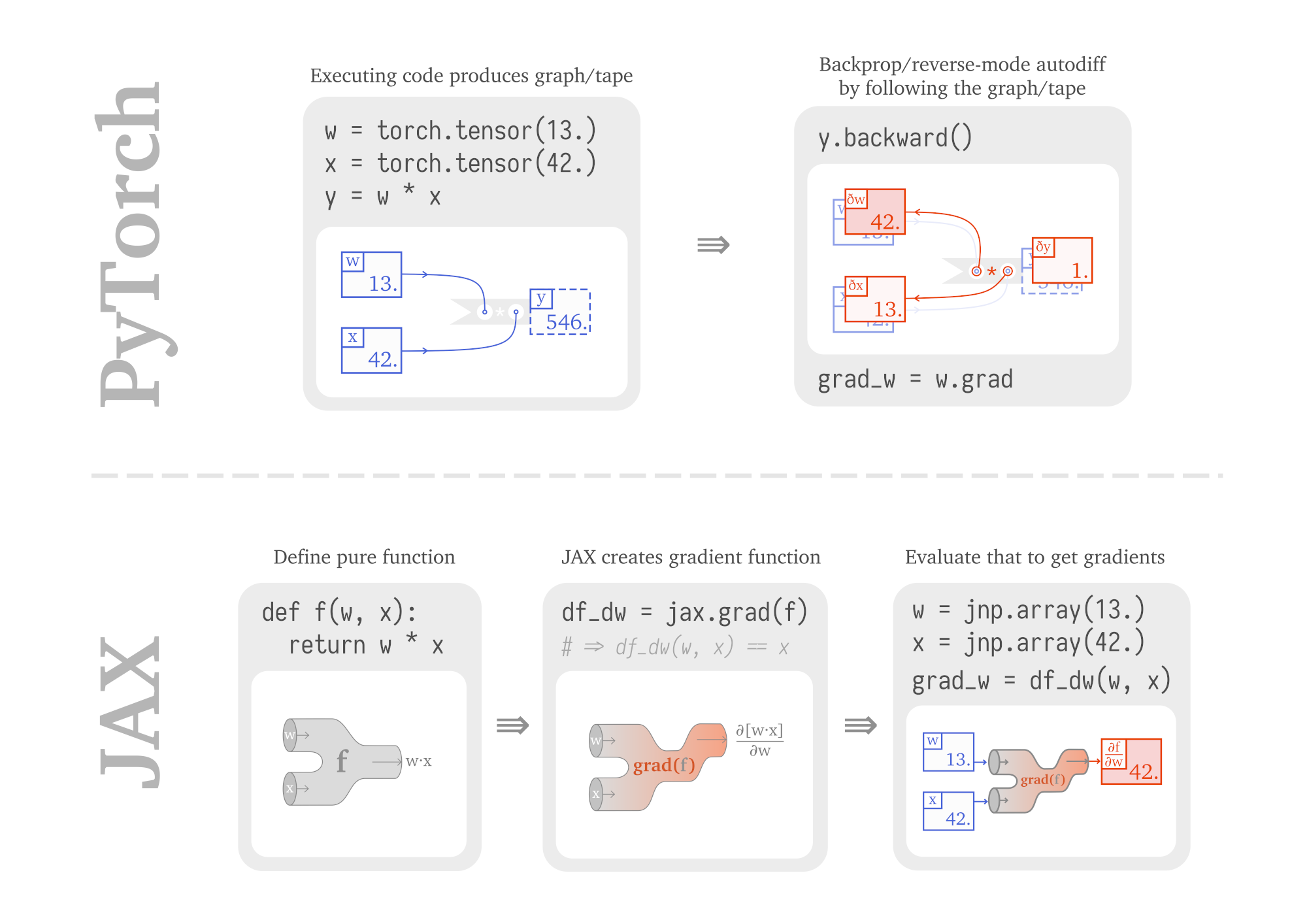
Exemple 1: autograd in pytorch
import torch
import torch.nn as nn
x=torch.ones(2,2)
x.requires_grad = True
y=x+2
z=y*y*3
out = z.mean()
out.backward()
print(x.grad)
Exemple 2: implementing backprop in numpy:
https://pytorch.org/tutorials/beginner/pytorch_with_examples.html#warm-up-numpy
- You have seen:
- Basic definitions & concepts
- loss, risk, regularization
- weights init, normalizations
- DL in practice: autograd, tricks, training loop, toolkits
Practice: code
- Objective:
- reminder: setup an XP protocol pipeline
- reminder: how to analyze results
- getting started with pytorch
- train, evaluate and analyze an MLP
- Copy-paste and analyse this code:
import numpy as np
import torch
import torch.nn as nn

class Net(nn.Module):
    def __init__(self,nins,nout):
        super(Net, self).__init__()
        self.nins=nins
        self.nout=nout
        nhid = int((nins+nout)/2)
        self.hidden = nn.Linear(nins, nhid)
        self.out    = nn.Linear(nhid, nout)

    def forward(self, x):
        x = torch.tanh(self.hidden(x))
        x = self.out(x)
        return x

def test(model, data, target):
    x=torch.FloatTensor(data)
    y=model(x).data.numpy()
    haty = np.argmax(y,axis=1)
    nok=sum([1 for i in range(len(target)) if target[i]==haty[i]])
    acc=float(nok)/float(len(target))
    return acc

def train(model, data, target):
    optim = torch.optim.Adam(model.parameters(), lr=0.001)
    criterion = nn.CrossEntropyLoss()

    x=torch.FloatTensor(data)
    y=torch.LongTensor(target)
    for epoch in range(100):
        optim.zero_grad()
        haty = model(x)
        loss = criterion(haty,y)
        acc = test(model, data, target)
        print(str(loss.item())+" "+str(acc))
        loss.backward()
        optim.step()

def genData(nins, nsamps):
    prior0 = 0.7
    mean0  = 0.3
    var0   = 0.1
    mean1  = 0.8
    var1   = 0.01

    n0 = int(nsamps*prior0)
    x0=var0 * np.random.randn(n0,nins) + mean0
    x1=var1 * np.random.randn(nsamps-n0,nins) + mean1
    x = np.concatenate((x0,x1), axis=0)
    y = np.ones((nsamps,),dtype='int64')
    y[:n0] = 0
    return x,y

def toytest():
    model = Net(100,10)
    x,y=genData(100, 1000)
    idx = np.arange(len(x))
    np.random.shuffle(idx)
    train(model,x[idx],y[idx])

if __name__ == "__main__":
    toytest()
What kind of model is this? Which non-linearity is used?
How is the data distributed?
Is a stochastic gradient descent used?
Do we need to shuffle the training data from one epoch to another?
Run it and plot the curves for the loss and for the accuracy
Adapt the code to create a test corpus with the same method as for the training corpus and evaluate your model
- Should you plot the validation loss, or the validation accuracy?
- Change the learning rate: what happens?
- with lr=1.0
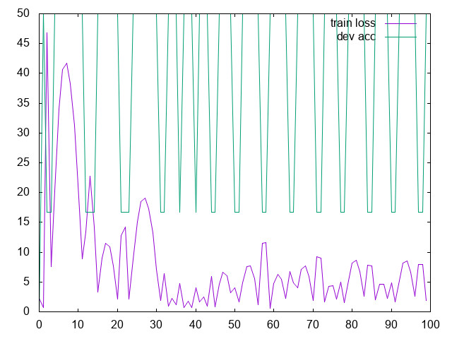
- Try to make your model overfit and not generalize well
- Add and tune L2 regularization so that it does not overfit any more
Correction
import numpy as np
import torch
import torch.nn as nn
class Net(nn.Module):
def __init__(self,nins,nout):
super(Net, self).__init__()
self.nins=nins
self.nout=nout
nhid = int((nins+nout)/2)
self.hidden = nn.Linear(nins, nhid)
self.out = nn.Linear(nhid, nout)
def forward(self, x):
x = torch.tanh(self.hidden(x))
x = self.out(x)
return x
def test(model, data, target):
x=torch.FloatTensor(data)
y=model(x).data.numpy()
haty = np.argmax(y,axis=1)
nok=sum([1 for i in range(len(target)) if target[i]==haty[i]])
acc=float(nok)/float(len(target))
return acc
def train(model, data, target, devx, devy):
optim = torch.optim.Adam(model.parameters(), lr=0.01)
criterion = nn.CrossEntropyLoss()
x=torch.FloatTensor(data)
y=torch.LongTensor(target)
idx = np.arange(x.size(0))
for epoch in range(1000):
np.random.shuffle(idx)
optim.zero_grad()
haty = model(x[idx])
loss = criterion(haty,y[idx])
acc = test(model, devx, devy)
print(str(loss.item())+" "+str(acc))
loss.backward()
optim.step()
def genData(nins, nsamps, mean0, mean1):
prior0 = 0.7
var0 = 0.1
var1 = 0.01
n0 = int(nsamps*prior0)
x0=var0 * np.random.randn(n0,nins) + mean0
x1=var1 * np.random.randn(nsamps-n0,nins) + mean1
x = np.concatenate((x0,x1), axis=0)
y = np.ones((nsamps,),dtype='int64')
y[:n0] = 0
return x,y
def toytest():
model = Net(100,10)
x,y=genData(100, 10, 0.3, 0.8)
devx,devy=genData(100, 100, 0.32, 0.8)
tex,tey=genData(100, 1000, 0.34, 0.8)
train(model,x,y,devx,devy)
if __name__ == "__main__":
toytest()
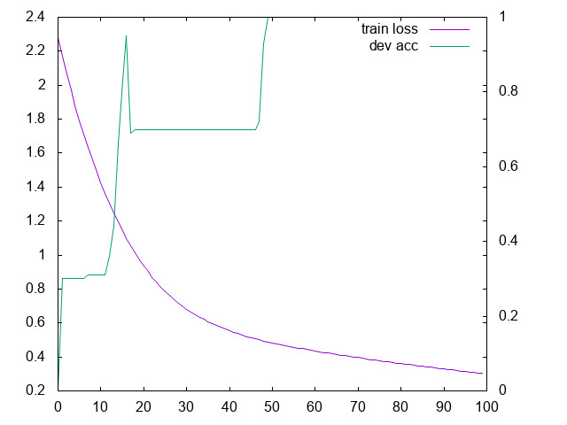
"""
python td1.py > tt
set y2tics
plot "tt" u 1 w l axis x1y1 t "train loss", "tt" u 2 w l axis x1y2 t "dev acc"
overfitting: lr=0.01, 10 training samples, 1000 epochs
L2 regul: weight_decay=1e-3
"""Brainstorming
Backprop vs. SGD
- Two algos are essential to optimize DNN: backprop and SGD
- what are their respective roles?
Differentiability
Let’s consider a DNN \(f(x_0)\), with a FF layer somewhere inside: \[y=relu(Wx)\]
- To optimize \(f\), we need its
derivative, but relu() is not differentiable!
- is it a problem?
- Let’s assume the following DNN+loss: \[f(x) = ||\max(g_1(x),g_2(x))-y||^2\]
- MAX is non-differentiable: can we learn \(f\) with SGD?
- Let’s assume the following DNN+loss: \[f(x) = ||int(Wx)-y||^2\]
- INT is non-differentiable: can we learn \(f\) with SGD?
Practice: design
- I assume you know MLP, CNN, RNN
- For each of the following dataset:
- what is the shape of the input tensor?
- which architecture would you build?
- “image denoising”:
- input = image
- output = denoised image
- “weather”:
- input = seq of (T°, atm pressure, light sensor)
- output = amount of rain
- “image captioning”:
- input = image
- output = text
- “speech recognition”:
- input = audio
- output = text
- “atari bot”
- input = screenshot + elapsed time
- output = joystick buttons
- “remaining useful life”
- input = sensors
- output = time until the machine breaks
TP
- Imagine a function of 2 variables, e.g. \(f(u,v)=u^2+v\) (don’t use this one!);
- Generate data from this function
- Train a feed-forward model
- Evaluate its performances
Losses
Losses
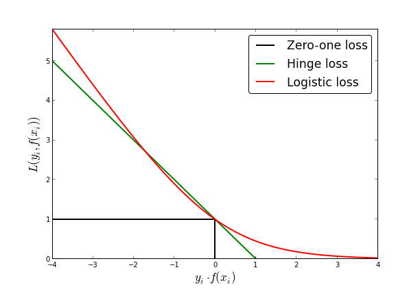
- Mean Square Error (MSE): \(l(\hat y,y) = || \hat y - y ||^2\)
- 0/1 loss
- Hinge loss
- Logistic loss
- Cross-Entropy loss: \(l(\hat y,y) = H(\hat y,y)\)
- Triplet (contrastive) loss
- …
0/1 and hinge loss
- Let \(y \in \{-1,1\}\) and \(f(x) \in R\)
0/1 and hinge loss
- 0-1 loss = classification error
- \(C = 1\) iff \(sgn(f(x)) \neq y\)
- not differentiable
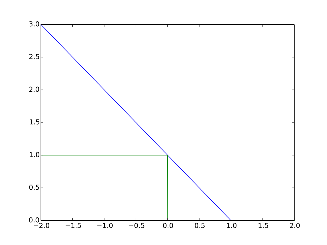
- Hinge loss: \(C = \max(0,1-yf(x))\)
- not differentiable at \(yf(x)=1\), but admits a subgradient
- “maximum-margin” classification
Logistic loss
- Logistic loss: \[\frac 1 {\ln 2} \ln(1+e^{-yf(x)})\]
- differentiable everywhere
Square error
MSE can be used also in classification:
with softmax and \(N\) classes: \[p(y_i|x) \simeq \frac {e^{\hat y_i}}{\sum_j e^{\hat y_j}}\]
assume 2 classes, 2 neurons; let \(i=\arg\max_{j\in \{0,1\}} y_j\) \[l(\hat y,y) = 2(1-y_i)^2\]
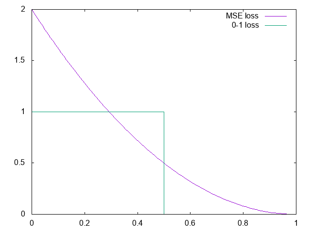
- Cross-entropy strongly penalizes the errors, so it’s sensitive to outliers
- But it’s equivalent to likelihood => default loss
Linear models
The Perceptron algorithm
Loss: Number of errors: \(1- \delta(y,sgn(f(x)))\)
Finds a hyper plane that separates training data
- Repeat until convergence:
- For \(t=1 \cdots n\):
- \(\hat y = sgn(f(x))\)
- if \(\hat y \neq y\) then \(\theta = \theta + yX\)
- For \(t=1 \cdots n\):
- Repeat until convergence:
Algorithm converges if training data separable (Novikoff,1962)
Limits of classification error loss
- Multiple solutions:

- Most of them will not generalize well !
Margin
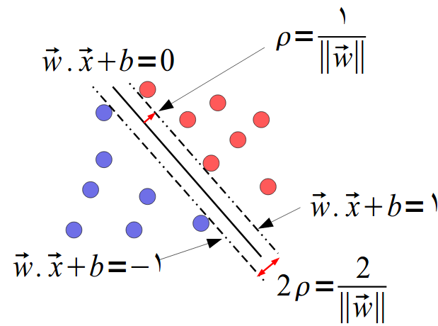
Margin
\(w\) is normal to the hyper-plane
distance \(r\) of any \(x\): \[w^T \left(x-yr\frac w {||w||} \right) + b=0\]
Solve for \(r\): \(r=\frac{y(w^Tx+b)}{||w||}\)
We choose a scaling of \(w\) and \(b\) s.t. \[y_i(w^Tx_i+b)\geq 1\]
with at least one equality, margin= \(\rho = \frac 2 {||w||}\)
Maximum Margin linear classifier
Find \(\theta\) that minimizes \(\frac 1 2 || \theta ||\) s.t. \[y_i X_i\theta \geq 1 ~~~ \forall i\]
= Quadratic programming problem
Gives a unique hyperplane as far as possible from training examples
The solution only depends on a subset of training examples that appear on the margin = the support vectors
Maximum Margin linear classifier
Limits:
if training data not separable, the hyperplane does not exist
even a single example can radically change the position of the hyperplane
SVM
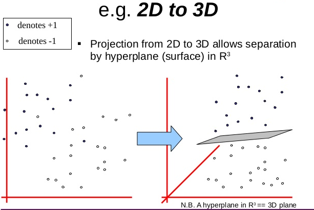
- Transform your input data with \(F(a)\) into a higher dimensional space so that it is linearly separable
- Kernel trick: Don’t explicit this transformation \(F(a)\) but use a kernel s.t. \(K(a,b)=F(a).F(b)\)
Unsupervised training
Generative model
Example:
- X = pressure (scalar)
- Y = will it rain ? (0 or 1)
Gaussian model for \(P(X|Y)\):
- Pick a centroid \(\mu_0\) and std dev \(\sigma_0\)
- Pick a centroid \(\mu_1\) and std dev \(\sigma_1\)
- Likelihood to observe this atm pressure when it rains: \[P(X|Y=1)=\frac 1 {\sqrt{2\pi}\sigma_1}e^{-\frac 1 2 \left( \frac{X-\mu_1} 2 \right)^2}\]
Unsupervised learning
Assume we don’t know any label \(Y\).
All we can do is fit a model on \(X\):
\[\hat\theta = \arg\max_\theta \prod_t P(X_t|\theta)\]
\[P(X|\theta)=\sum_y P(X,Y=y|\theta) = \sum_y P(X|Y=y,\theta)P(Y=y)\]
Unsup. training of the generative model
Assume \(P(Y)\) uniform: we only need to maximize \[\prod_t \sum_i \frac 1 {\sqrt{2\pi}\sigma_i}e^{-\frac 1 2 \left( \frac{X_t-\mu_i} 2 \right)^2}\]
- When we change \(\theta\), this likelihood change
- So there exists an optimum that can be found for \(\theta\)
Discriminative model
Linear model: \[\hat y = w x + b\]
We want a probability: logistic regression: \[P(Y=1|X) = \frac 1 {1+e^{-(wx+b)}}\]
Unsup training of discriminative model
\[P(X|\theta)=\sum_y P(X,Y=y|\theta) = \sum_y P(Y=y|X,\theta)P(X)\]
Getting \(P(X)\) out of the sum: \[P(X|\theta)=P(X)\]
The observation likelihood does not depend on the parameters !
So it is impossible to maximize it…
Evaluation
holdout split
- Our objective is to predict new (never seen) samples
- So we never evaluate on the training set
- Best approach: holdout data split
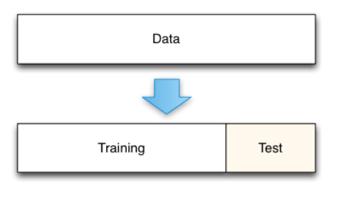
- Main issues:
- Penalizing for small datasets
- Experiments must never be run several times on the test set !! \(\rightarrow\) contamination
Cross-validation
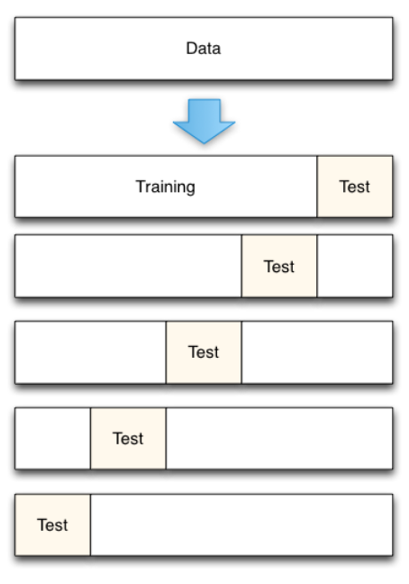
Cross-validation
How many folds ?
- Few: biased error estimates with low variance
- Many (leave-one-out): unbiased error estimate but high variance
- Practical: 5-folds or 10-folds
- X-val gives you 1 training + 1 “test” accuracy
- What if you want to change the LR? Test another model?
- You may use x-val to train the model + train the hyper-parm
- But how good is your model? What if you don’t have any other test corpus?
Hyper-parameter tuning
Best option: further split the training set on 2 subsets: training + development
Alternative: nested cross-validation
For each test fold i:
    - For each possible values of hyper-parms:
        For each dev fold j != i:
            - train on remaining folds
            - evaluate on dev fold j
        Average results on all dev folds
    - Pick the best hyper-parms
    - Retrain model on all folds but i
    - Evaluate on test fold
Average results over test folds- OK, you can train parms and hyper-parms, and evaluate your procedure
- but what is your final model?
- Is your procedure still as good on 9/10th or 10/10th of the corpus?
- and it’s super slow…
Evaluation metrics
Standard classification metric: accuracy \[ acc = \frac{N_{OK}} {N_{tot}}\]
Question: on the same test set,
- classifier C1 gives 71% of accuracy
- classifier C2 gives 73% of accuracy
- Is C2 better than C1 ?
Confidence interval
- Standard statistical hypothesis test:
- Hyp H0: C2 is not better than C1
- Accuracy is a proportion: compute 95%-Wald confidence interval: \[p \pm 1.96 \sqrt{\frac {p(1-p)} n}\]
with \(n=\) nb of samples in the test corpus.
Example with 1000 examples in test:
- acc(C1) \(\in \{68.2\%; 73.8\%\}\)
- acc(C2) \(\in \{70.2\%; 75.7\%\}\)
So we can not conclude that C2 is better than C1
Detection
- True positive (TP): \(f(x)=+\) and \(y=+\)
- False positive (FP): \(f(x)=+\) but \(y=-\)
- True negative (TN): \(f(x)=-\) and \(y=-\)
- False negative (FN): \(f(x)=-\) but \(y=+\)
Precision: \(p = \frac {TP}{TP+FP}\)
Recall: \(r = \frac {TP}{TP+FN}\)
Accuracy: \(a = \frac {TP+TN}{TP+TN+FP+TN}\)
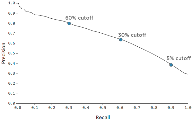
Detection threshold
We may want to be sure that every positive detected is really positive
Adjust decision threshold:
- pos. iff \(f(x)>\tau\)
Precision-recall curve:
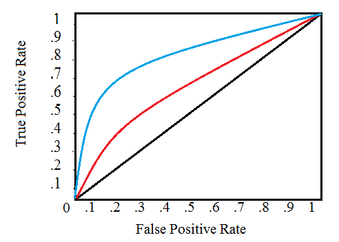
ROC curve
- True positive rate = recall
- False positive rate = \(\frac{TN}{TN+FP}\)
Receiver Operating Characteristic:
References
https://web.engr.oregonstate.edu/~tgd/classes/534/slides/part9.pdf
http://www-bcf.usc.edu/~gareth/ISL/ISLR%20Seventh%20Printing.pdf
-
- generalization, bias-variance
- nested cross-validation
- confidence intervals
Descent methods
- When we want to optimize some function (risk)
- But we don’t have a closed-form solution
\(\rightarrow\) Descent methods
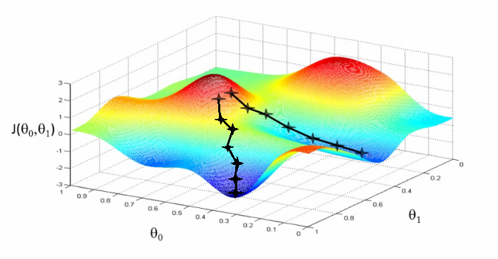
Finding the descent direction
Any \(\Delta x\) that verifies:
\[\Delta x^T \nabla f(x) < 0\]
is a descent direction.
- For small \(t\): \[f(x+t\Delta x) \simeq f(x) + t\Delta x^T \nabla f(x)\]
Gradient descent
How to find the descent direction ?
Simplest approach: Gradient descent: \[\Delta x = -\nabla f(x)\]
For strictly convex functions, we have linear convergence: \[f(x^k)-p \leq c\left( f(x^{k-1})-p \right)\]
with \(0 < c < 1\)
- At each iteration, the error is multiplied by a number less than 1, so eventually converges to 0
Problem 1 with gradient descent
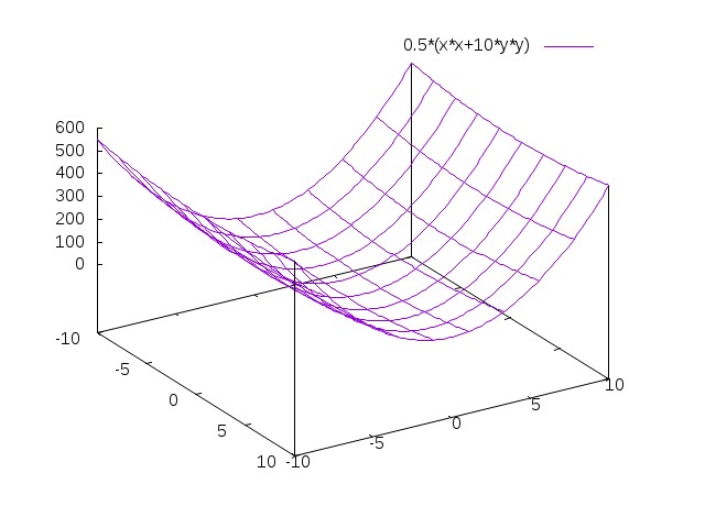
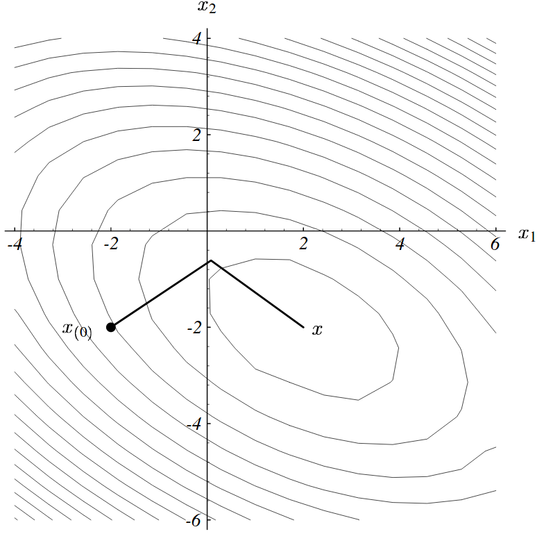
\[f(x)=\frac 1 2 (x_1^2 + ax_2^2)\]
\[\nabla f(x) = [ x_1 , ax_2 ]\]
From the point (1,1), the steepest descent is (-1,-a)
But we know \(\min f\) is in (0,0) \(\rightarrow\) optimal direction (-1,-1)
Problem 1 with gradient descent
Problem 1 with gradient descent
- Conversely, the optimal direction is found in one step of \(a=1\):
- Gradient descent is not invariant to linear transformations!
So scaling of inputs is very important !
- If GD slow, try rescaling your data and the parameters
- You can use a fixed step size, but have to tune it
Newton’s method
Multiply the gradient with the inverse Hessian:
\[\Delta x = -H(x)^{-1} \nabla f(x)\]
\[H(x)=\nabla^2 f(x) = \frac {\partial^2 f(x)}{\partial x \partial x^T}\]
Handles relative scaling between dimensions, and so is invariant to linear changes of coordinates
If \(f(x)\) quadratic, gives the global optimum direction
But it is not invariant to higher order (e.g. quadratic) changes of coordinates
It may be very costly (\(O(N^3)\) with \(N\)=nb of dimensions) to solve the linear system \(H(x)^{-1}\nabla f(x)\)
Quasi-Newton method
Approximate \(f\):
\[f^k(x+v)=f(x)+\nabla f(x)^T v + \frac 1 2 v^T B_k v\]
The direction of the descent is:
\[\Delta x = -B_k^{-1} \nabla f(x)\]
\(B_k\) is an approximation of the Hessian that is continuously updated
See also Kylov methods to approximate Hessian
BFGS method
Special case of Quasi-Newton method: Broyden, Fletcher, Goldfarb and Shanno.
–
BFGS method
\[s_k = x_{k+1} - x_k\]
\[y_k = \nabla f(x^{k+1})-\nabla f(x^k)\]
\[\rho_k = \frac 1 {y_k^T s_k}\]
\[F_{k+1} = (I-\rho_k s_k y_k^T) F_k (I-\rho_k y_k s_k^T) + \rho_k s_k s_k^T\]
Descent direction \(F_k \nabla f(x)\) can be computed in \(O(N^2)\)
Problem 2 with gradient descent
- For quadratic fcts, search directions are successively orthogonal
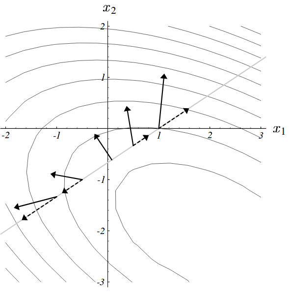
Problem 2 with gradient descent
- This leads to longer paths than what could be expected
Conjugate gradient
- Eliminate all of the error along one axis in one step
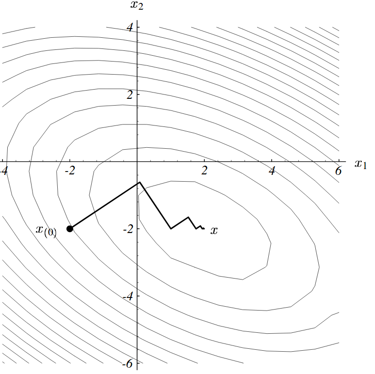
Problem 3 with gradient descent
As well as conjugate gradient:
- In non-convex space, do not generalize well
- Solution: simulated annealing
- Requires to compute the gradient of the error over the full corpus
Stochastic Gradient Descent
Assume the function to minize has the form: \[f(x)=\frac 1 T \sum_t^T f_t(x)\]
This is the case for
- maximum likelihood training
- empirical loss minimization
Stochastic Gradient Descent
Standard Gradient Descent:
\[x \leftarrow x - t\nabla f(x)\]
SGD approximates the gradient with the gradient at a single sample:
\[x \leftarrow x - t\nabla f_i(x)\]
In practice:
- Shuffle the dataset at the beginning of each epoch
- Iterate over all samples in the dataset
SGD convergence
There are proofs that, under relatively mild assumptions, and when the learning rates \(t\) decrease with an appropriate rate, then SGD converges almost surely to a global minimum when the function is convex, and otherwise to a local minimum.
SGD + back-propagation is used to train all deep neural nets
Recent research works suggest that SGD is so successful because such an approximation of the gradient strongly regularizes the learning process.
SGD with momentum
Momentum:
\[\Delta x \leftarrow \alpha \Delta x - t \nabla f_i(x)\]
- There’s a “memory” / “inertia” of the previous update
- This prevents oscillations
Other SGD extensions
decay: the learning rate decreases over time
Adagrad: different learning rate per dimension
RMSProp: uses a running average of recent gradients per dimension
Adam: enhancements of RMSProp
mini-batch SGD: rule of thumb: use 32, 64, 128 or 256
Reminders: ConvNet
Limits of feed-forward networks
Example: Check whether a person appears in a photo
- reduced B&W photo: 300x200 = 60k inputs
- several layers, for instance 60k X 1000 X 10 neurons
- 60M parameters (=connections) !
- Sample 1: the person appears on the top-left of the photo
- Sample 2: the same person appears on the bottom-right of the photo
- Common information between both samples is lost !
Reduce number of parameters by sharing connection weights:
- Exploit the structural properties within data
- E.g., for images: invariance to translation
- So we can use the same set of weights at various positions of the image
- \(\rightarrow\) convolutional networks
- E.g., for speech: Markov property of the signal
- \(\rightarrow\) recurrent networks
- E.g., for graph data:
- \(\rightarrow\) graph convolutional networks
2D convolution
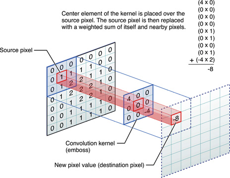
Kernel size = 3x3
- Input image \(I\)
- Kernel \(K=\) matrix of size \(h \times w\)
\[(I * K)_{x,y} = \sum_{i=1}^h \sum_{j=1}^w K_{ij} \cdot I_{x+i-1,y+j-1}\]
- Assume the input has \(d\) channels (red/green/blue), the kernel dimensions are extended accordingly
- A bias and an activation are also typically used:
\[conv(I,K)_{x,y} = \sigma\left(b+\sum_{i=1}^h \sum_{j=1}^w \sum_{k=1}^d K_{ijk} \cdot I_{x+i-1,y+j-1,k}\right)\]
Stride / Shift
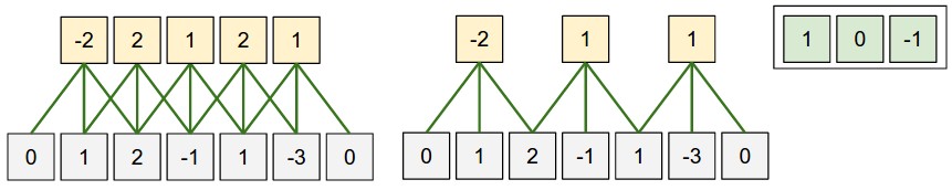
Stride = 1 …………………. Stride = 2
Receptive field = 3
Padding
Kernel size 3x3, stride 2, padding 1

Adding filters
- Apply 5 convolutions \(\rightarrow\) 5-dim vector:
Adding filters
Pooling
With appropriate kernel size, padding and stride1, the resulting “blurred image” has the same size as the input image
We want to compress the information and reduce the layers size progressively down to the final layer:
- Option 1: remove padding, increase stride
Pooling
- Option 2: downsampling = pooling
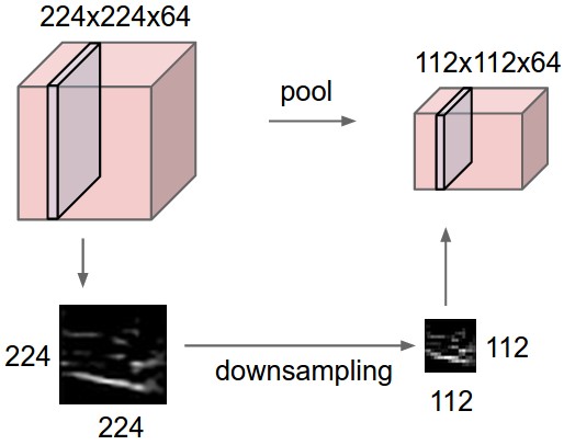
Pooling
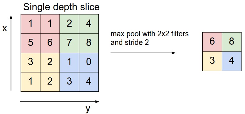
Max pooling = pick the max value within a filter size
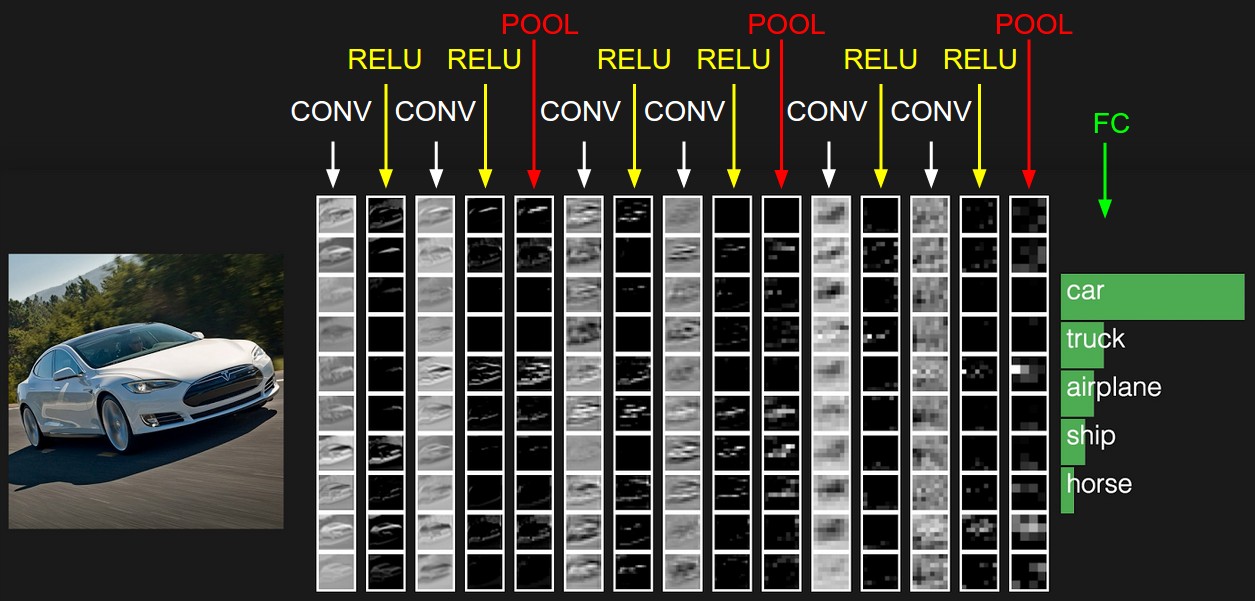
ConvNet = stacking of various types of layers
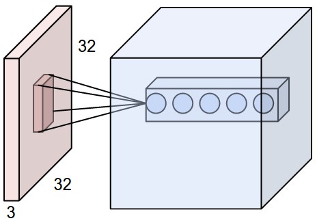
Extensions: 1x1 convolution
![]()
- reduce dims: 200x200x50 \(\rightarrow\) 200x200x\(N_f\)
- add another non-linearity, with few parameters (deeper net)
Extensions: dilated convolution
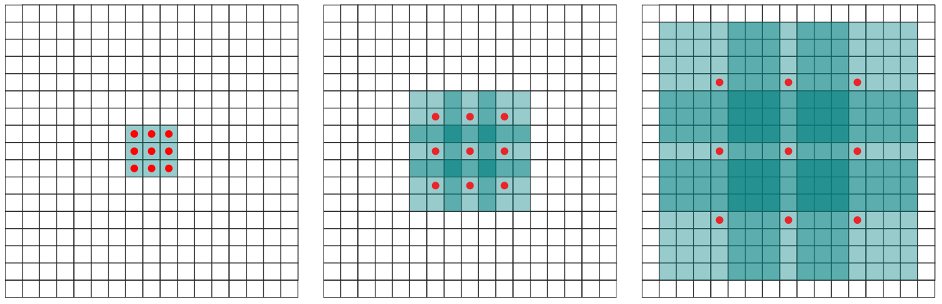
- skip 0, or 1, or 3 pixels
- increase receptive field
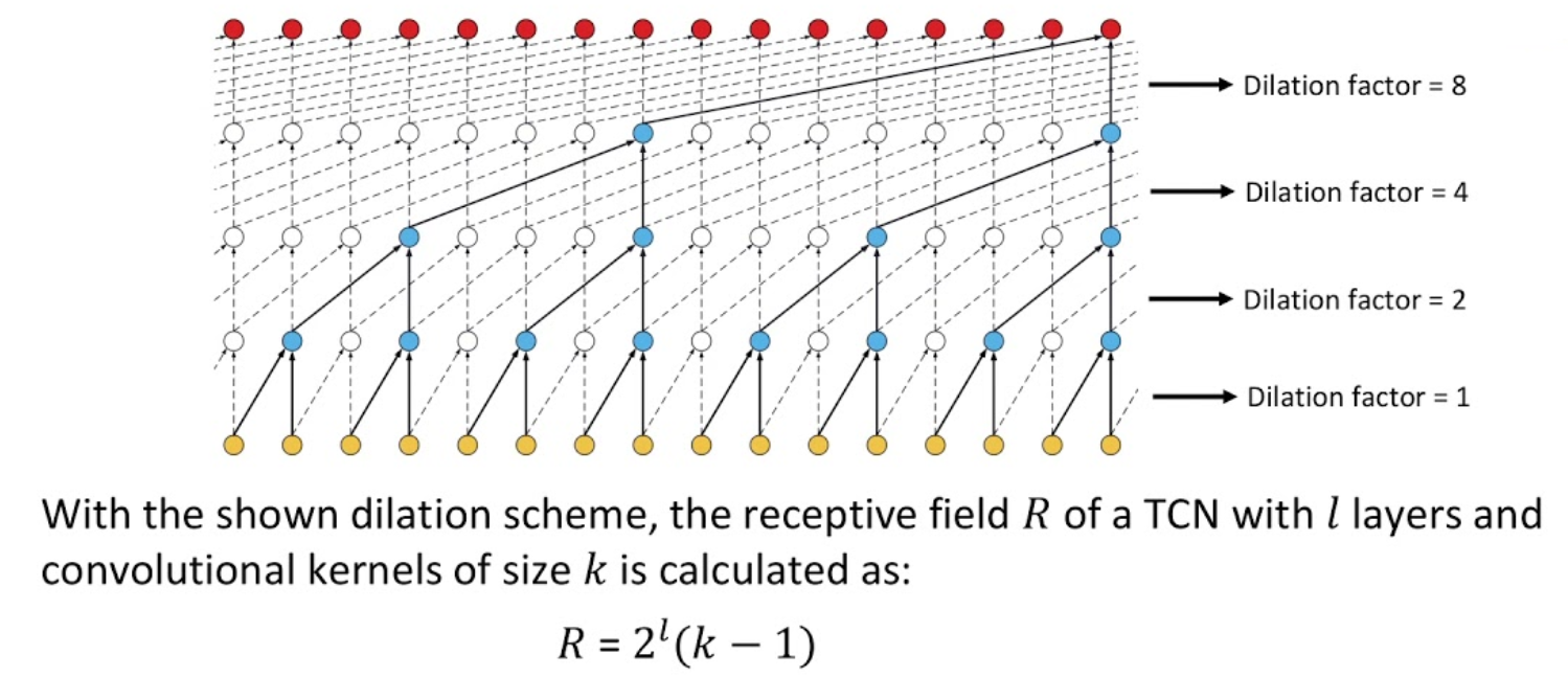
Extensions: temporal convolution
ConvNet architectures
INPUT -> [[CONV -> RELU]*N -> POOL?]*M -> [FC -> RELU]*K -> FC- Prefer a stack of small filter CONV to one large receptive field CONV layer
Hyper-parameter choice
input layer should be divisible by 2: 32, 64, 96, 224, 384, 512
conv layer use small filters (3x3, at most 5x5)
pool layer: usually 2x2 with stride 2
Model Zoo in Image Processing
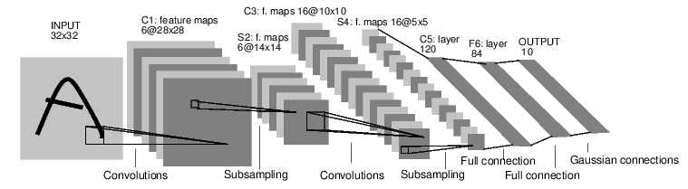
LeNet
- Yann Lecun 1990
AlexNet
- Alex Krizhevsky, Ilya Sutskever, Geoff Hinton, 2012

GoogleNet
- Szegedy et al., 2014
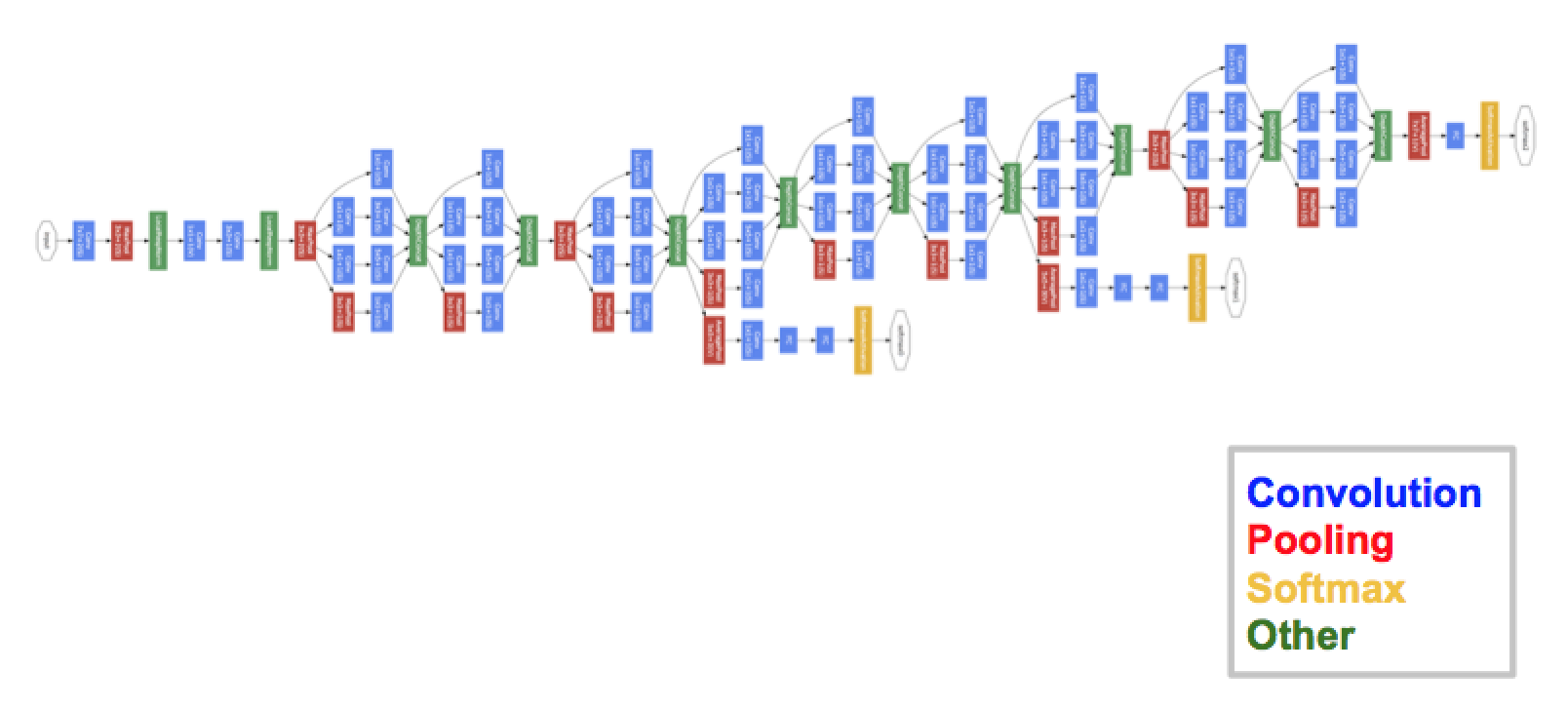
GoogleNet
Inception module:
- Let the model choose:
- compute multiple transformations: 1x1-conv, 3x3-conv, 5x5-conv, 3x3-pool
- Reduce dimensionality:
- by adding 1x1-convolutions
VGGNet
Karen Simonyan, Andrew Zisserman, 2014
Classical architecture but much deeper
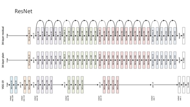
ResNet
- Kaiming He et al., 2015
DenseNet
G. Huang et al., 2016
each layer directly connected to all following layers
Model Zoo in Natural Language Processing
- Use 1D-convolutions instead of 2D-convolutions
- shift the kernel along the time axis only
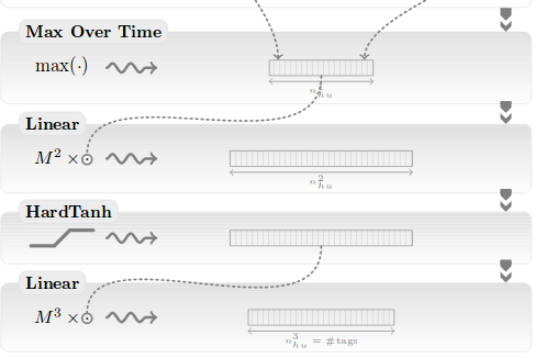
Collobert et al., 2011
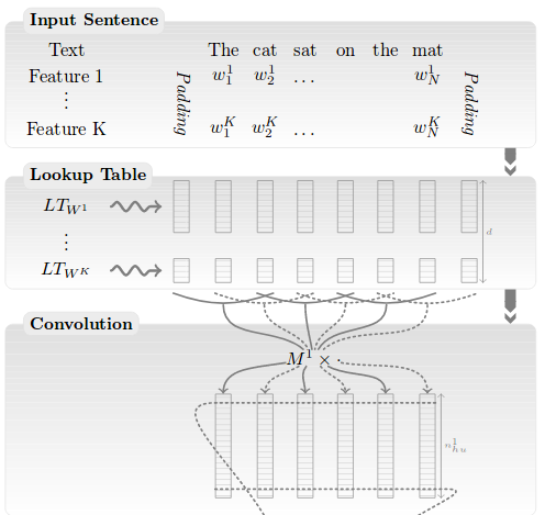
Collobert et al., 2011
- Lookup table = Word Embeddings
- assign a single vector \(\vec w \in
R^{100}\) to every word in the voc.
- e.g. \(\vec w_{le}\), \(\vec w_{chat}\), \(\vec w_{chien}\)
- whenever word \(w\) occurs in the
input, this vector \(\vec w\) is
inserted as input
- e.g. “le chat le chien” \(\rightarrow\) \((\vec w_{le}, \vec w_{chat}, \vec w_{le}, \vec w_{chien})\)
- the real values in these vectors are trained by back-propagation
- assign a single vector \(\vec w \in
R^{100}\) to every word in the voc.
- The following convolutions use 100 input channels
Collobert et al., 2011
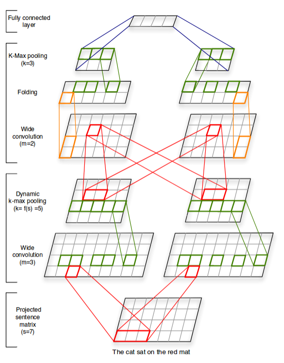
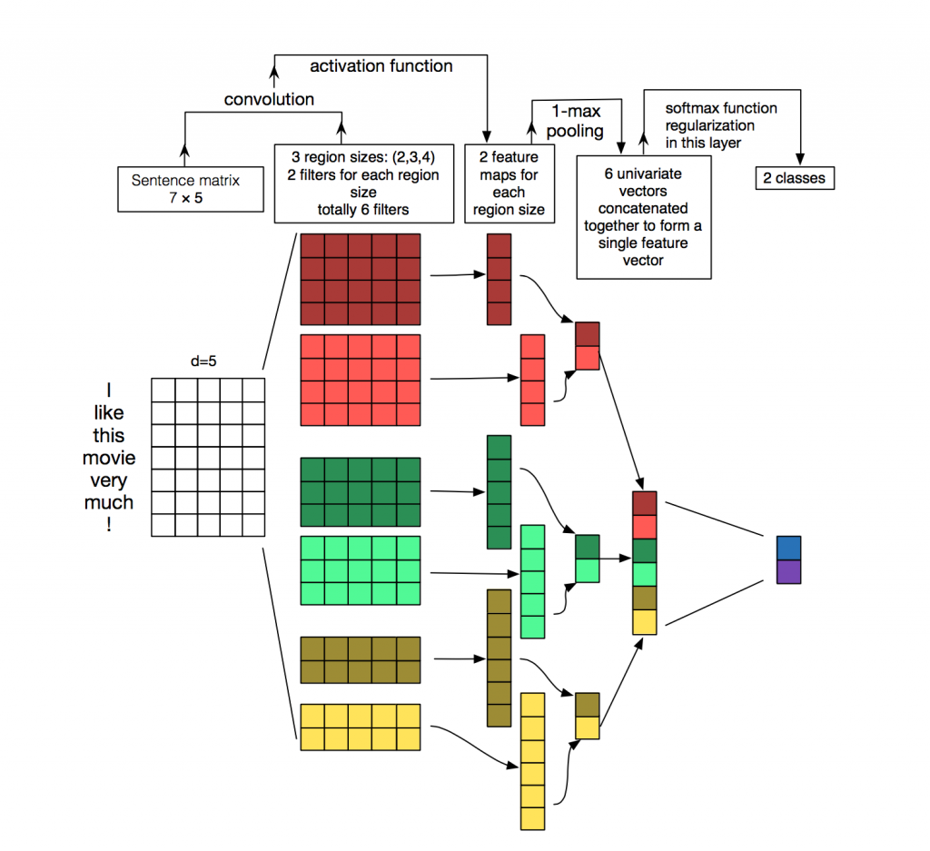
Wide and deep CNN
Yoon Kim, 2014
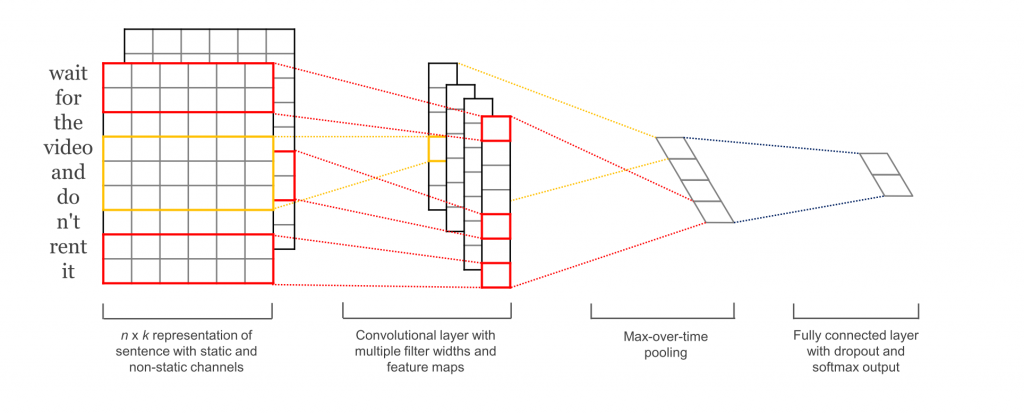
Not very deep, but extremely efficient !
Kalchbrenner, 2014
Zhang et al., 2015
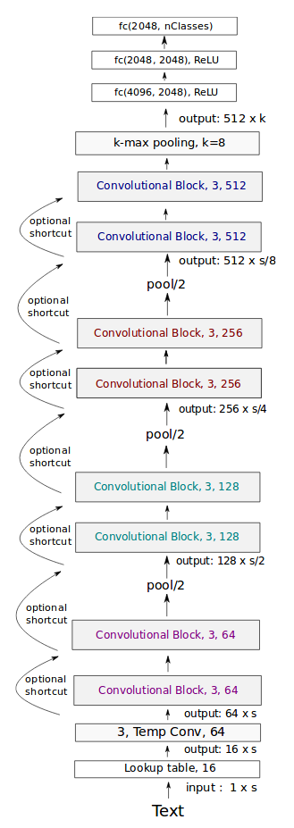
Very deep CNN: Conneau (FAIR), 2017

Transfert learning
- ConvNets are reusable amongst multiple tasks
- Nobody retrains a CNN from scratch
- Remove the last layer of ImageNet ConvNet
- … or fix the N first layers
Practice: CNN
- Download Meteo data
- Goal = predict the next T° given a seq of T°
- train on 2019, test on 2020
- Objectives:
- template code for CNN & time series
- use of Dataset & DataLoader
- explore underfitting/overfitting
- understand sources of variability
- Data: convert to tensor, then to Dataset, then to DataLoader:
# trainx = 1, seqlen, 1
# trainy = 1, seqlen, 1
trainds = torch.utils.data.TensorDataset(trainx, trainy)
trainloader = torch.utils.data.DataLoader(trainds, batch_size=1, shuffle=False)
testds = torch.utils.data.TensorDataset(testx, testy)
testloader = torch.utils.data.DataLoader(testds, batch_size=1, shuffle=False)
crit = nn.MSELoss()- Model: simple CNN with a linear regression layer:
class Mod(nn.Module):
    def __init__(self, nhid):
        super().__init__()
        self.cnn = nn.Conv1d(in_channels=1, out_channels=nhid, kernel_size=3)
        self.mlp = nn.Linear(nhid,1)

    def forward(self,x):
        # x = B, T, d
...- Every day, the CNN predicts the next day T°:
- \(X\) is a tensor (Batch, Time, Dim) = (1, 365, 1)
- WARNING! With a kernel 3, the CNN shall predict:
- day 4 from days 1,2,3
- day 5 from days 2,3,4 …
- loss = MSE
- TODO1: write the forward() method of your model: useful fcts:
- print(x.shape) : print the dims of the tensor x
- x = x.view(10,2) : change the dims of x (e.g., from (20,) to (10,2))
- x = x.transpose(1,2) : x (a,b,c) becomes (a,c,b)
- test it with:
mod=Mod(h)
x=torch.rand(1,7,1)
y=mod(x)
print(y.shape)- compute MSE on test:
def test(mod):
    mod.train(False)
    totloss, nbatch = 0., 0
    for data in testloader:
        inputs, goldy = data
        haty = mod(inputs)
        loss = crit(haty,goldy)
        totloss += loss.item()
        nbatch += 1
    totloss /= float(nbatch)
    mod.train(True)
return totloss- Training loop:
def train(mod):
    optim = torch.optim.Adam(mod.parameters(), lr=0.001)
    for epoch in range(nepochs):
        testloss = test(mod)
        totloss, nbatch = 0., 0
        for data in trainloader:
            inputs, goldy = data
            optim.zero_grad()
            haty = mod(inputs)
            loss = crit(haty,goldy)
            totloss += loss.item()
            nbatch += 1
            loss.backward()
            optim.step()
        totloss /= float(nbatch)
        print("err",totloss,testloss)
print("fin",totloss,testloss,file=sys.stderr)- The Main:
mod=Mod(h)
# visualize the model
for n,p in mod.named_parameters(): print(n,p.shape)
print("nparms",sum(p.numel() for p in mod.parameters() if p.requires_grad))
train(mod)- Step 1: copy/paste + complete this code and run a training
- check convergence!
- Step 2: compare and analyze \(h=1\), \(h=100\)
- Step 3: rerun multiple times: what’s the variability and why?
Correction
import sys
import torch.nn as nn
import torch
import numpy as np

dn = 50.
h=10
nepochs=100

with open("meteo/2019.csv","r") as f: ls=f.readlines()
# divides by dn to normalize inputs (temp is below dn=50 degree)
# removes last elt (:-1) because it has no label (cannot predict next temp)
trainx = torch.Tensor([float(l.split(',')[1])/dn for l in ls[:-1]]).view(1,-1,1)
# we want to predict y=x[3] from x[0,1,2] (because kernel size = 3)
# so the label of the first batch should be x[mod.kern], and so on...
trainy = torch.Tensor([float(l.split(',')[1])/dn for l in ls[3:]).view(1,-1,1)

with open("meteo/2020.csv","r") as f: ls=f.readlines()
testx = torch.Tensor([float(l.split(',')[1])/dn for l in ls[:-1]]).view(1,-1,1)
testy = torch.Tensor([float(l.split(',')[1])/dn for l in ls[3:]).view(1,-1,1)

# trainx = 1, seqlen, 1
# trainy = 1, seqlen, 1
trainds = torch.utils.data.TensorDataset(trainx, trainy)
trainloader = torch.utils.data.DataLoader(trainds, batch_size=1, shuffle=False)
testds = torch.utils.data.TensorDataset(testx, testy)
testloader = torch.utils.data.DataLoader(testds, batch_size=1, shuffle=False)
crit = nn.MSELoss()

class Mod(nn.Module):
    def __init__(self,nhid):
        super(Mod, self).__init__()
        self.cnn = nn.Conv1d(1,nhid,3)
        self.kern = 3
        self.mlp = nn.Linear(nhid,1)
        self.relu = nn.ReLU()

    def forward(self,x):
        # x = B, T, d
        # we want B, d, T (see doc Conv1d)
        xx = x.transpose(1,2)
        y=self.cnn(xx)
        y=self.relu(y)
        B,H,T = y.shape
        yy = y.transpose(1,2)
        # yy = B, T, d
        y = self.mlp(yy.view(B*T,H))
        y = y.view(B,T,-1)
        return y

# mod=Mod(h)
# x=torch.rand(1,7,1)
# print(x.shape)
# y=mod(x)
# print(y.shape)
# exit()

def test(mod):
    mod.train(False)
    totloss, nbatch = 0., 0
    for data in testloader:
        inputs, goldy = data
        haty = mod(inputs)
        # goldy = B, T, d
        loss = crit(haty,goldy)
        totloss += loss.item()
        nbatch += 1
    totloss /= float(nbatch)
    mod.train(True)
    return totloss

def train(mod):
    optim = torch.optim.Adam(mod.parameters(), lr=0.001)
    for epoch in range(nepochs):
        testloss = test(mod)
        totloss, nbatch = 0., 0
        for data in trainloader:
            inputs, goldy = data
            optim.zero_grad()
            haty = mod(inputs)
            loss = crit(haty,goldy)
            totloss += loss.item()
            nbatch += 1
            loss.backward()
            optim.step()
        totloss /= float(nbatch)
        print("err",totloss,testloss)
    print("fin",totloss,testloss,file=sys.stderr)

mod=Mod(h)
print("nparms",sum(p.numel() for p in mod.parameters() if p.requires_grad),file=sys.stderr)
train(mod)
RNN zoo
- Deep learning works with any function/program; but standard “blocks”
are often used to make it easy:
- feed-forward == Multi-Layer Perpectron
- convolution: ConvND, dilated, temporal-conv…
- recurrent: RNN, LSTM, GRU…
- graph-CNN, recursive, memory-nets…
- auto-enc, enc-dec, VAE…
- siamese, contrastive, GAN…
- flow-based, diffusion…
- attention, transformers, MoE…
Recurrent neural networks
http://www.wildml.com/2015/09/recurrent-neural-networks-tutorial-part-1-introduction-to-rnns/
http://karpathy.github.io/2015/05/21/rnn-effectiveness/
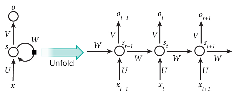
- \(x\) = observation/input; \(o\) = output
- \(s\) = hidden neuron = represents the “state” (=memory)
\[s_t = f(Ux_t + W s_{t-1})\]
RNN training
Back-Propagation Through Time:
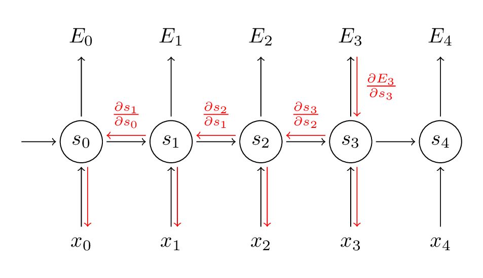
Back-Propagation Through Time
- Key diff with standard backprop: the gradients sum at every time step
Exemple: gradient with respect to output 3: \[\frac{\partial E_3}{\partial W} = \sum_{k=0}^3 \frac{\partial E_3}{\partial \hat y_3} \frac{\partial \hat y_3}{\partial s_3} \left( \prod_{j=k+1}^3 \frac {\partial s_j}{\partial s_{j-1}} \right) \frac{\partial s_k}{\partial W}\]
Vanishing gradient
Derivative of the \(tanh\) activation:
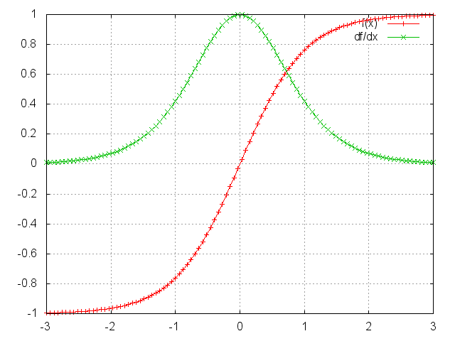
The gradient of the activation is often close to 0
When many such gradients are multiplied, the gradient becomes smaller and smaller, negligeable
After some time steps, no more training is possible
Exploding gradients are also possible, but can be solved with clipping
Solutions to vanishing gradient
- Careful initialization of the \(W\) matrices
- Careful tuning of regularization
- Use ReLU activations instead of sigmoid/tanh
- Bypass activations as in LSTM or GRU cells
LSTM
- Computes the new state \(s_{t+1}\)
from the previous state and input using 3 gates:
- input gate: how much of the input-derived state we let through
- forget gate: how much of the previous state we let through
- output gate: how much of the overall state will be passed out
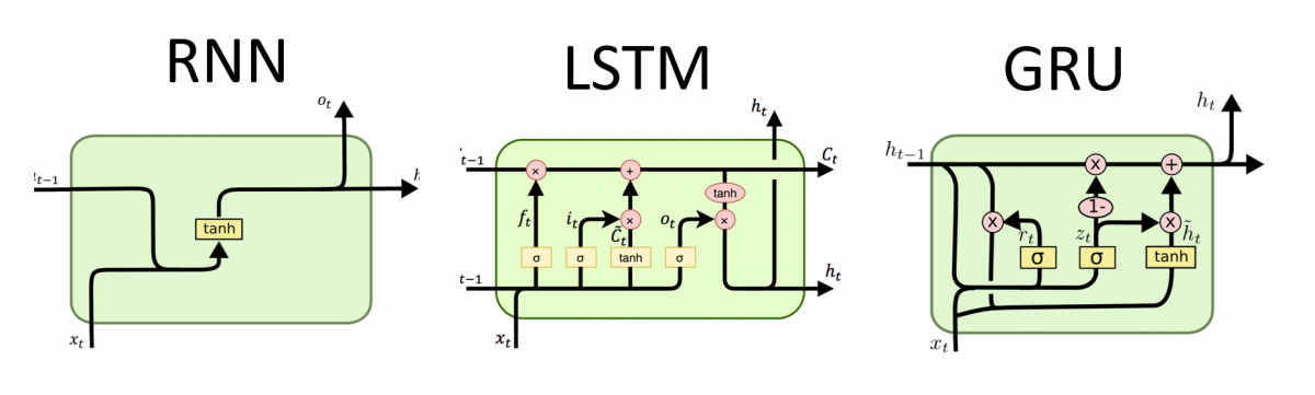
Vanishing gradient
- RNN
- Bi-directional
- stacked LSTM
- hierarchical
- with attention
- seq2seq
Sequence-to-Sequence (Seq2Seq)
Cho et al., 2014
Other models zoo
- vision: U-Net, R-CNN, ViT, YOLO, FCN, Segnet…
- time series: Temporal-CNN…
- audio: Wav2Vec, Wavenet, tacotron…
- GAN: cycleGAN, WassersteinGAN, VQGAN, DCGAN, StyleGAN, StarGAN, SRGAN, StudioGAN, BigGAN, InfoGAN, CipherGAN…
- attention: MemNET, NTM, RETRO…
Other models zoo
- AE: VAE, GMVAE
- Graph: GCN…
- multimodal: diffusion…
- Unsupervised: deep clustering, MUSE, UNIT, tabnet, BEGAN, BYOL, DeepSAD, DEC
- Deep-RL
Take home
- Why not always use MLP ?
- parameter sharing
- inductive bias & data struct.
- CNN: inv. by translation
- RNN: decreasing dep. to time
- Transformers: no info bottlenecks
Git cheat sheet
- git = software to version your code
locally:
- stores every version in the history (compressed in ./.git/)
- enables collaborative edition
- can sync with 1+ repos: github.com, gitlab.com, gitbucket…
Quick set-up
- set-up an account on github.com with an SSH key
- create a repo on github.com
- download the repo on your laptop once:
git clone git@github.com:...- before any working session, sync from github:
git pull origin mainQuick set-up
- edit the code locally
- tell git about every new file you want to version:
git add myfile.py- every 30’, save your edits in the local history:
git commit -am "I fixed the bug"- and upload them to github:
git pull origin main
git push origin main
Troubleshooting
- NEVER copy/move/rename/delete a file without “git”, rather do:
git rm oldfile.py
git mv oldfile.py newfile.py- NEVER create/clone a repo in or below another repo dir
Troubleshooting
- by default, “git pull” is cautious and never
destroys information
- if several people modified different lines, it’ll merge all modifications
- if concurrent modifs of the same lines, it’ll refuse to merge: conflict
- solve a conflict:
- both versions of conflicting lines are saved in the file
- just edit the one you want to keep; then:
git add file_that_was_in_conflict.py
git commit -am "conflict solved"
git push
Troubleshooting
- If you’re lost / nothing works as expected:
- just clone a fresh version from github of the repo in another directory
- work again from this fresh version
- never copy any file into this fresh version !!!
- Tips:
- “git pull” should be run very frequently (as many times as you want)
- you can run “git pull” at any time: nothing is destroyed!
- “git commit” + “git push” frequently to avoid conflicts
- the longer time btw 2 syncs, the more problems
- never copy/move any file in a git directory!
- Tips:
- Many docs use the command “git add .”
- Never do that!
- Better to select manually each important file you want to add, one by one
- Don’t version large files!! (pdf, zip, mp4, mp3…)
- see “git lfs” if you really want them to be versioned
- Many docs use the command “git add .”
- Tips:
- Learn git with one of the many online tutos: