Transformers, scaling law
Attention models
- Intuition of hard attention:
- Imagine a long text about history
- You observe a new short text about year 1515
- Your model shall focus / pick info from the relevant passage in the long text
- How do you know if a passage is relevant?
- compute a similarity btw passage and query
- similarity = dot-product
- Select only the passage with largest similarity
- Intuition of soft attention:
- Pick info from all passages, but weight them by their relevance
- relevance = normalized similarity (by softmax)
- Attention can be applied to many cases:
- long texts, banks of vectors, output sequences of RNN…
- more generally:
- Let be a bank of vectors (\(k_i\),\(v_i\))
- Let \(q\) be a new vector: what is its value?
- Compute the distance between \(q\) and every \(k_i\): \(q \cdot k_i\)
- Normalize with softmax: \(\alpha_i = Softmax (q \cdot k_i)\)
- Compute the target value: \(v = \sum_i \alpha_i v_i\)
Self-attention
- attention of every \(x_t\) against all \(\{x_{t'}\}_{1\leq t'\leq T}\)
- so every token generates a new “smoothed” version of itself, smoothed by all other tokens
- so self-attention can be viewed as a layer that transforms an input seq into an output seq of the same length
- pb: does not consider position at all (for now)
- distance is irrelevant
- relies on tokens content only
- nb of parameters does not depend on seq length
- For each target token:
- Compute its dot-product with every other token
- Normalize them all with softmax
- Replace its vector by the weighted average of all tokens
- Can be done with 2 inner FOR loops, or with matrix algebra
- Let \(X_t\) be an embedding of input token
- 3 matrices (the parameters) are used to transform \(X_t\) into
- a query vector: \(Q_t = X_t^T W_Q\)
- a key vector: \(K_t = X_t^T W_K\)
- a value vector: \(V_t = X_t^T W_V\)
- Computes the distances between \(Q_t\) and every \(K_{t'}\): \[a_{t'} = Q_t \cdot K_{t'}^T\]
- Normalize to get the attention vector: \[\alpha = Softmax(a_1,\cdots,a_T)\]
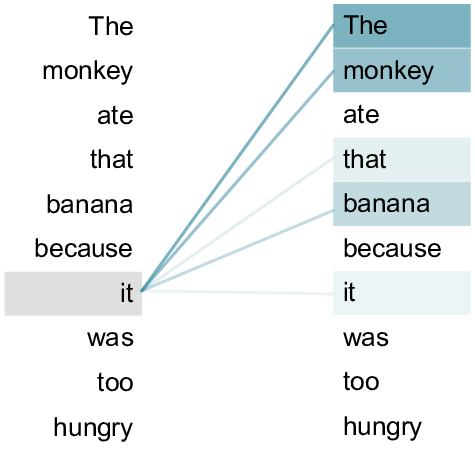
- gives degree of relatedness btw token \(X_t\) and all other tokens
- Often represented by a heat map over the words of the sentence
Expressing dot-product with matrices:
\(Q=\begin{bmatrix} ~~~~~Q_1^T~~~~~\\ \hline \cdots\\ \hline ~~~~~Q_T^T~~~~~ \end{bmatrix}\) \(K=\begin{bmatrix} ~~~~~K_1^T~~~~~\\ \hline \cdots\\ \hline ~~~~~K_T^T~~~~~ \end{bmatrix}\)
\[\alpha = Softmax(QK^T)\]
- warning: softmax over which dimension?
Scaled dot-product
- \(q\) and \(k\) are \(d_k\)-dimensional vectors
- assume \(q_i\) has mean 0 and var 1
- then \(q\cdot k\) has var \(d_k\)
- so we scale the dot-product to get var=1:
\[\alpha = Softmax\left( \frac{QK^T}{\sqrt{d_k}} \right) \]
- We give each token a repr \(V_{w}\)
- Pool them into a matrix for the seq: \(V = [V_{w_1},\dots,V_{w_N}]^T\)
- We replace every target token repr by the average over its context (weighted by \(\alpha\))
\[ V' = Softmax\left( \frac{QK^T}{\sqrt{d_k}} \right) V\]
- Caution about the matrices dimensions !
Multi-head self-attention
- Repeat with different \(W_Q,W_K,W_V\) to get multiple heads
![]()
Positional Encodings
- Self-attention gives the same repr when you shuffle the words !
- Inject information about position through a vector that encodes the position of each word
- Naive approaches:
- \(p=1,\dots,N\): not normalized + never seen N
- \(p=0,0.06,\dots,1\): \(\Delta p\) depends on sentence length
- Better approach:
- inspired by spectral analysis
- positions are encoded along sinusoidal cycles of various frequencies
\[p_t^{(i)} = \begin{cases} sin(w_k \cdot t), \text{if }i=2k \\ cos(w_k \cdot t), \text{if }i=2k+1 \end{cases}\]
with \(d\) encoding dim and
\[w_k = \frac 1 {10000^{2k/d}}\]
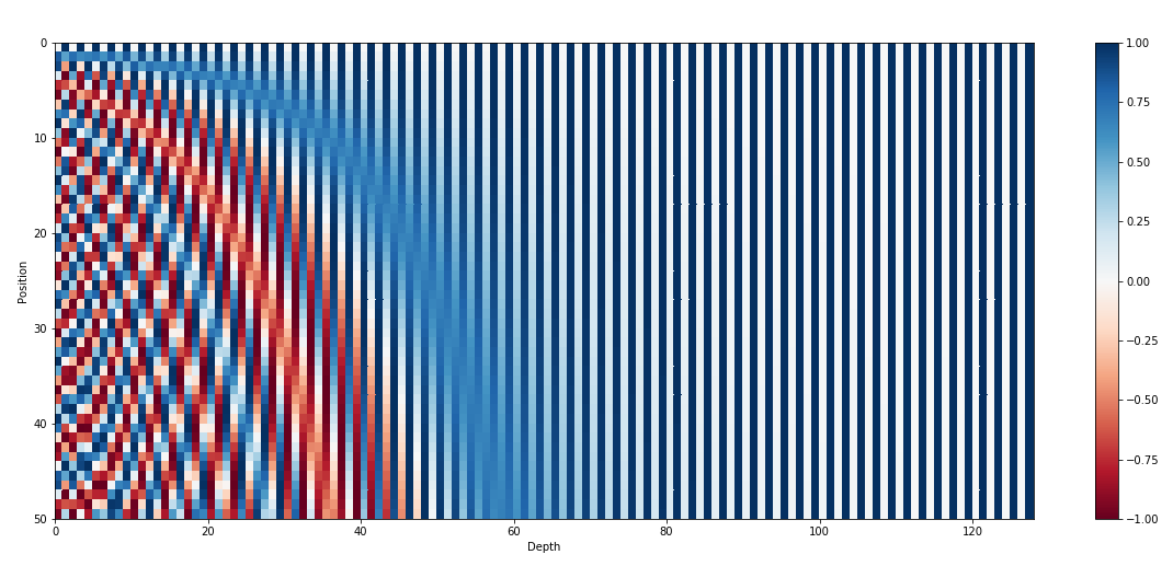
- Remarks:
- by giving positional encodings the same dimension as word embeddings, we can sum them together
- most positional information is encoded in the first dimensions, so summing them with word embeddings enable the model to “let” the first dimensions free of semantics and dedicate them to positions.
- Other types of positional encodings:
- train 1 embed per absolute position
- Alibi
- Rotary
- …
Transformer: “Attention is all you need”
![]()
![]()
- Add a normalization after self-attention
- parametric center+scale 1 vec across dimensions
- better gradient (cf paper)
![]()
- Add another MLP to transform the output
- Add residual connections: smooth loss landscape
- Stack this block \(N\) times
![]()
- Stack this block \(N\) times
- not so much about abstraction
- about redundancy
- about having multiple paths
- The transformer is designed for Seq2Seq
- So it contains both an encoder and decoder
- Same approach for decoder
- with cross-attention from encoder to decoder matching layers
- with masks to prevent decoder from looking at words \(t+1, t+2\dots\) when predicting \(t\)
- GPT family: only the decoder stack
- BERT family: only the encoder stack (+ classifier on top)
- T5, BART family: enc-dec
- Implementation details of the transformer:
- great resource:
- see The annotated transformer
QCM4
| Q001 | Q002 | Q003 | Q004 | Q005 | Q006 | Q007 | Q008 | Q009 |
|---|---|---|---|---|---|---|---|---|
| 77.00% | 69.00% | 69.00% | 85.00% | 100.00% | 0.00% | 62.00% | 92.00% | 54.00% |
| Q010 | Q011 | Q012 | Q013 | Q014 | Q015 | Q016 | Q017 | Q018 |
| 100.00% | 38.00% | 77.00% | 62.00% | 46.00% | 23.00% | 77.00% | 85.00% | 38.00% |
Self-supervised training
- Manual annotations into supervised classes (e.g., emotion) is costly
- Find an auxiliary task to learn representations
- This task must force the model to learn useful information
- Ex. for GPT:
- Language modeling taks:
- predict the next word \(p(x_t|x_0,\dots,x_{t-1})\)
- Ex. for BERT:
- Masked language modeling:
- predict a masked word \(p(x_t|x_0,\dots,x_{t-1},x_{t+1},\dots,x_T)\)

- Quest of models able to “absorb” huge datasets
- Vision, speech: ConvNets (2012)
- “Absorb” ImageNet
- Higher layers == more abstract visual features
- 2021: CoAtNet-7 (Conv + Atten): 2.4 million parameters
- Vision, speech: ConvNets (2012)
- Quest of models able to “absorb” huge datasets
- Language: transformers (2018)
- “Absorb” the written web
- 2021: Wu Dao 2.0: 1.75 trillion parameters (10x GPT3)
- Language: transformers (2018)
- Big NLP models absorb:
- lexicon, syntax, semantics of NL
- facts described in the web:
- cooking recipies
- historical events
- famous people
- …
- Big NLP models are trained to “complete” sentences
- Try it:
- GPT3 API
- AI dungeon
- Huggingface hub
- Bing chat, you.com…
- Try it:
Exploiting representations
- With Zero-Shot learning
- With few-shot learning
- As frozen embeddings
- With fine-tuning
Using LLMs: Zero-Shot Learning
- “Give me a recipe to cook bacon”
- “place the bacon in a large skillet and cook over medium heat until crisp.”
- “The main characters in Shakespeare’s play Richard III are”
- “Richard of Gloucester, his brother Edward, and his nephew, John of Gaunt”
(More on ZSL later…)
Using LLMs: Few-Shot Learning

- can be done on a laptop
- requires very few annotated data
- a bit better than ZSL
Using LLMs: as frozen embeddings

- can be done on a laptop
- requires some annotated data
- gives good results
Using LLMs: with fine-tuning

- can be done on a desktop
- requires some annotated data
- gives the best results
Instruction finetuning
- Foundation model = pretrained generic LLM that can be finetuned on various tasks
- Instruction finetuning = pretrained LLM finetuned on instructions (QA, procedures, chat)
- RLHF / DPO = finetuned LLM aligned with human values
- pretrained LLM:
- has all the knowledge inside
- is not able to chat, answer questions…
- instruction finetuned LLM:
- no more knowledge, but can interact with human
- aligned LLM:
- does not say “bad” things
Zero-Shot learning
You may query LLM without further training:
- “Is this review positive or negative? Review: this
is the best cast iron skillet you will ever buy”
- “Positive”
- “A is the son’s of B’s uncle. What is the family
relationship between A and B?”
- “cousins”
- “A is the son’s of B’s uncle. What is B for A?”
- “brother”
- “On a shelf, there are five books: a gray book, a
red book, a purple book, a blue book, and a black book. The red book is
to the right of the gray book. The black book is to the left of the blue
book. The blue book is to the left of the gray book. The purple book is
the second from the right. Which book is the leftmost book?”
- “The black book”
Prompt programming
- is the art of designing prompt to perform a task
- Prompting may be viewed as a way to constraint the generation
- You may describe the task
- You may give examples (few-shots)
- You may give an imaginary context to “style” the result
- How to describe the task:
- direct task description
- proxy task description
- Direct task description:
- “translate French to English”
- Can be contextual:
- “French: … English: …”
- Direct description can combine tasks the model must know:
- “rephrase this paragraph so that a 2nd grade can understand it, emphasizing real-world applications”
- Proxy task description
This is a novel written in the style of J.R.R. Tolkien’s Lord of the Rings fantasy novel trilogy. It is a parody of the following passage:
“S. Jane Morland was born in Shoreditch …”
Tolkien rewrote the previous passage in a high-fantasy style, keeping the same meaning but making it sound like he wrote it as a fantasy; his parody follows:
- Few-shot prompts:
English: Writing about language models is fun. Roish: Writingro aboutro languagero modelsro isro funro. English: The weather is lovely! Roish:
- “chain of thoughts”:
- “think step by step…”
- decompose a difficult task into steps
- only works with large models (>100GB)
- Efficient to solve math problems
- New types of prompts discovered regularly:
- Program of thoughts
- Tree of thoughts
- Analogical prompting
- Prompting to verify its output
- “Take a deep breath”
- “This is important for my career”…
- Going further:
- Other applications of these models:
- Vision Transformers (ViT)
- protein folding (Nature: Jumper et al. 2021)
- Code generation: Github Co-pilot
- Image generation: DALL-E
Transformers
- Ubiquitous in Natural Language Processing
- Dominating in Image Processing:
![]()
les LLM, une nouvelle recherche empirique
Des observations aux prémisses de théories
- Observations:
- Mémorisation, compression, structuration et généralisation
- Capacités émergentes
- Embryons de théories: Passage à l’échelle
- Lois de Chinchilla
- Grokking
- Double descente
- Transitions de phases, singularité…
- Why are transformers so good?
- Enable the model to scale:
- with reasonable depth (<100)
- demultiply the number of “paths” information can flow
- but still share parameters across paths
- RNN: cannot scale (training cost)
- CNN: information only compressed through a “local funnel”, no paths
- MLP: not efficient (lack of inductive bias)
Scaling laws
Scaling property of LLMs
- scaling = if you add parameters, it can store more information
- controlled by measuring its performances on tasks
- scaling law = power law = \(y(x) = ax^{-\gamma} +b\)
- metric = test loss
- \(\gamma\) = slope
Baidu paper 2017
GPT3-175b paper 2020
- emergence of In-Context Learning !
- provide examples of a task in the context, the output mimics the examples
Scaling laws for Neural LM 2020
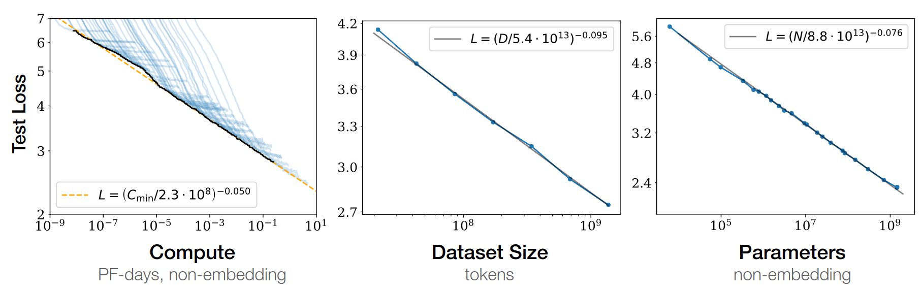
Open-AI 2020
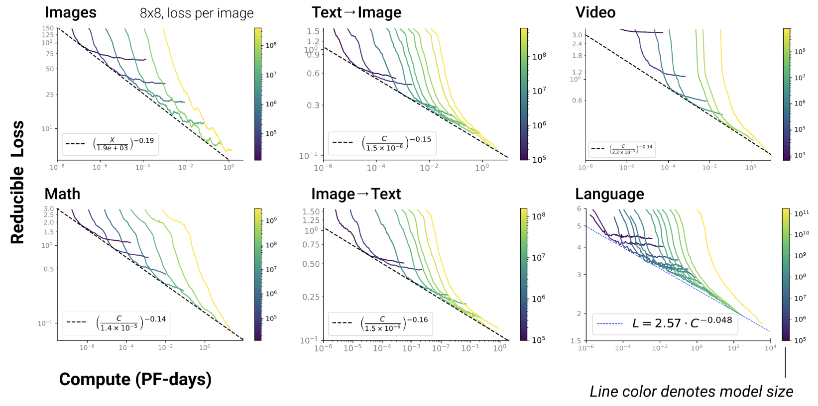
- RL, protein, chemistry…
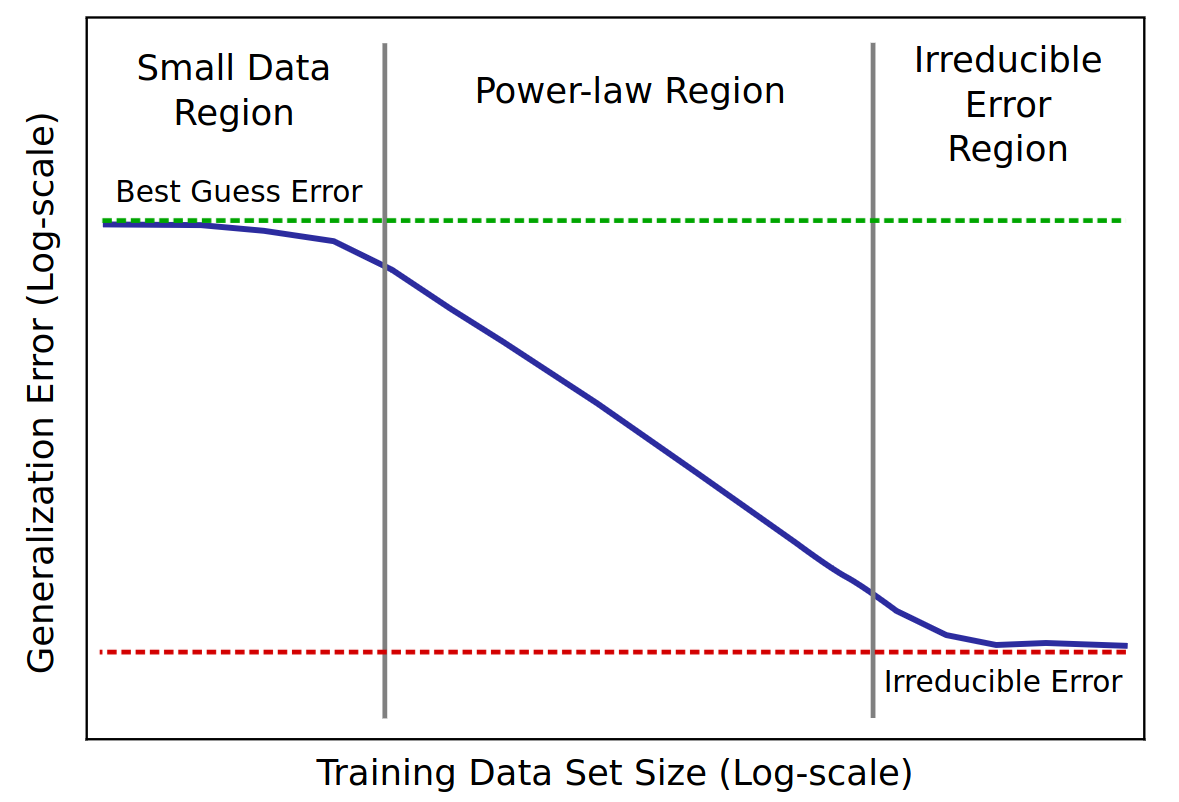
- Scaling exist since long in ML Paper on learning curves
- But reducing test loss is linked to emergent abilities in
transformers
- Such emergence never been observed in ML before
Chinchilla paper 2022
- GPT3: train on 300b tokens, and scale parameters up
- given fixed FLOPS, optimal balance btw dataset / parameters
- Lesson: need more data!
\(L(N)=\frac A {N^\alpha}\)
- \(N\) = dataset size
- \(\alpha \simeq 0.5\) (was 0.05 in GPT3 paper)
![]()
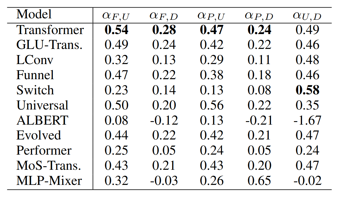
- Any really useful enhancement of transformers since 2017?
- FlashAttention
- Pre-layer norm
- Parallel feed-forward and attention
- Rotary + Alibi positional encodings
Anthropic paper 2022
- smooth scaling results from combination of abrupt emergences
Importance of scale
- Large number of parameters are required to simply store all the factual information
- But LLMs also compress information
- and to efficiently compress, the LLM needs to store the algorithm instead of the data
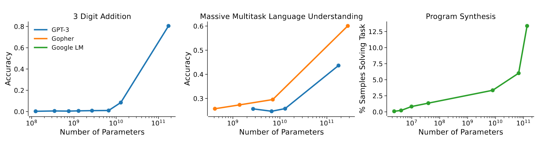
- Some new abilities of transformers only emerge after a certain
scale:
- Nobel-prize Philip Anderson: “Emergence is when quantitative changes in a system result in qualitative changes in behavior.”
- for language: “Emergent Abilities of Large Language Models”
Emergence of few-shot prompting

Emergence of other abilities

- for vision: “Emerging Properties in Self-Supervised Vision Transformers”
- emergence of semantic segmentation without supervision

Scaling with Mixture of Experts
- Sparse activations per input
- Each input goes through same amount of computation, but different paths
- \(N\) experts \(E_i(x)\)
- One gating network: \(p_i(x) = \frac {e^{h(x)_i}}{\sum_{j=1}^{M<N} e^{h(x)_j}}\)
- First success in Translation: Switch Transformer
- replace FFN in transformers with MoE
- choose single highest-prob expert
- Issue: unstable training; remedy:
- selective precision: 32 bits for exp computation, 15 bits for others
- reduce init scale
- more dropout for experts
- MoE requires auxiliary loss to balance the load across experts (Shazeer et al., 2018)
Scaling with finetuning
- Small data regime: finetuning better than training

but forgetting; hard to inject new knowledge
Opening LLMs
- a.k.a. foundation models
- a list, with openness level, available here
Useful links
- You have seen:
- evolution from RNN to transformers
- details of attention, self-attention, positional embeddings
- hints at the reasons of their success
- scaling law: we’re still far from limits
- new scaling directions: sparse MoE
LLM costs
QCM5
| Q001 | Q002 | Q003 | Q004 | Q005 | Q006 | Q007 | Q008 | Q009 |
|---|---|---|---|---|---|---|---|---|
| 17% | 100% | 75% | 50% | 33% | 50% | 17% | 83% | 92% |
| Q010 | Q011 | Q012 | Q013 | Q014 | Q015 | Q016 | Q017 | Q018 |
| 17% | 50% | 58% | 33% | 17% | 50% | 33% | 42% | 92% |
Training costs
- LLama2-70b: 5M€, 2M GPU.h
- 1 epoch training:
- RedPyjama v2: 30T tokens
- assume 100 toks/s on GPU, how long?
- Hyper-parms tuning ???
- cf. muP paper
- Training huge LLM is very difficult: The LLM training handbook
Inference costs
- Autoregressive generation
- practice: estimate time/token when generating on your laptop
- Serving many requests
- OpenAI API has become a “standard” for self-serving
- benchmarks like HELM rely on this API
- evaluating one model on HELM: $10k
- distillation
- unstructured pruning
- see “Lottery ticket hypothesis”
- result: sparse model, not GPU-compliant
- structured pruning
- see “Sheared Llama”
- keep similar architecture
- quantization
- parameters: usually 16 bits, can get 4 bits
- see GPTQ, bitsandbytes, AWQ
- exercice: how much RAM used with?
m = AutoModelForCausalLM.from_pretrained("facebook/opt-350m", load_in_4bit=True)- optimization (ollama, lama.cpp, vLLM, localai.io…)
- often quantizes 4 bits by default
- C++ code to run inference / serve LLM
Finetuning costs
- Parameter-efficient finetuning
- adapters
- soft prompts
- prefix tuning
- low-rank adaptation
- Main LLM parameters are frozen
- Adapters
- add a new sub-layer at every LLM layer
- see Adapter hub
- Soft prompts
- Bypass the embedding layer and start the input with a few parameter vectors
- see tuto
- Prefix tuning
- Same as soft prompt, but add new vectors at input of every layer
- variants: P-tuning…
- Finetuning with qLoRA
- Full finetuning requires VRAM = 4x nb parameters
- Better:
- quantize in 4 bits, freeze all parameters, just train 16 bits-LoRA
- See HF how to
Practice: self-attention
- Create 3 random pytorch tensors, with dimension n: they represent your input sequence of length 3: \(X_1,X_2,X_3\)
- Create 3 random matrices for queries, keys and values
- Compute, in one operation, all the key tensors from all input tensors.
- Do the same for values and queries.
- Compute the dot-product between the queries Q and all keys K1,K2,K3
- You should get 3x3 attention scores (scalar)
- Normalize these attention scores with a softmax
- Compute the sum of the input value tensors, weighted by their corresponding attention score
- You obtain the output sequence of vectors.
- Goal: perform classification after attention
- Compress this variable-length final sequence into a single fixed-size vector with max-pooling
- Add a final classification layer to predict 2 classes and put all this inside a pytorch nn.Module model
Limitations
- Generate random scalar sequences:
- class A: the sequence is composed of observations uniformely sampled between 0 and 1
- class B: the sequence is composed of observations uniformely sampled between 1 and 2
- Train your self-attentive classifier
- Analyze
- Generate random sequences:
- class A: the first half of the sequence is composed of observations uniformely sampled between 0 and 1, and the second half between 1 and 2
- class B: the first half between 1 and 2, and the second half between 0 and 1
- Train your self-attentive classifier
- Analyze
Refs
http://jalammar.github.io/illustrated-transformer/
Practice: attention
Buggy attentive RNN
class ModelAtt(Model):
  def __init__(self):
      super(ModelAtt, self).__init__()
      qnp = 0.1*np.random.rand(self.hiddensize)
      self.q = nn.Parameter(torch.Tensor(qnp))

  def forward(self, x):
      batch_size = x.size(0)
      hidden = self.init_hidden(batch_size)
      steps, last = self.rnn(x, hidden)
      alpha = torch.matmul(steps,self.q)
      alpha = nn.functional.softmax(alpha,dim=1)
      weighted = torch.mul(steps, alpha)
      rep = weighted.sum(dim=1)
      out = self.fc(rep)
return out, alpha- 2-Classif: perturbed sinusoid up vs. down
def f(x,offset):
    return 0.3*math.sin(0.1*x+offset)+0.5

nex=100
nsteps=50
input_seqs = []
target_seqs = []
for ex in range(nex):
    offset = np.random.rand()
    input_seq=[f(x,offset) for x in range(nsteps)]
    cl = np.random.randint(2)
    target_seqs.append(cl)
    if cl==0: perturb = 0.05
    else: perturb = -0.05
    pos=np.random.randint(25,45)
    for t in range(pos,pos+5): input_seq[t]+=perturb
    input_seqs.append(input_seq)

input_seq = torch.Tensor(input_seqs)
input_seq = input_seq.view(nex,nsteps,1)
target_seq = torch.LongTensor(target_seqs)- Train attentive RNN:
- Use 10000 epochs, LR=0.0001 and RMSprop optimizer
- Use the CrossEntropyLoss() instead of the MSELoss() to learn the two classes
- Does it learn to predict the two classes correctly? Is learning stable?
- After training, plot both the input curve and the attention weights, for the first 5 curves: does attention correctly spots the perturbation?
- Try without the offset: what happens? Does attention spots the perturbation? Explain.
- Try to find better hyper-parameters so that convergence is faster.
- Modify the training loop so that random curve generation is generated directly inside the training loop: there is no more any epoch, but only an infinite sequence of random batches: what happens?
- Try with longer vs. shorter and smaller/bigger perturbations: in which cases does it work or not? How sensitive is the approach to perturbations?
Transformers zoo
- See huggingface hub: 77k models!
- NLP:
- BERT, RoBERTA, ALBERT, GPT2, GPTJ, GPT-NeoX, BART, T5, T0pp…
- French: CamemBERT, FlauBERT
- Translation: T5, opus-MT, WMT, MT5
- QA: longformer, gelectra, XLM
- Summarization: BART, Pegasus, BigBird…
- multilingual: XLM-R, MGPT, Bloom…
- Image classification:
- ResNet, CLIP-ViT, MIT-B2, SWIMi, DEIT…
- Image segmentation:
- Segformer, Detr-ResNet, Maskformer…
- Image2image:
- MirNET (enhance), cond-GAN, BiT, DiffusionCLIP, StableDiffusion…
- Speech reco: wav2vec, HuBERT, Whisper…
- Audio classif: XLSR, wav2vec, music-generation…
- Text2Speech: Amadeus, TTS-hifigan, Tacotron2, Jets…
- Audio2Audio: MTL-mimic, DCCR, DPRNN, Sepformer, DCUNet…
- Text2image: Stable-diffusion, Waifu-diffusion, AI-dreamer, DALLE-Mega, BigGAN, DOODAD…
- Image2Text: ViT-GPT2, TROCR, Donut, Flamingo…
- Document-QA: LayoutLM
- RL: decision-transformer, PPO, MLAgents…
Practice: huggingface / fairseq
how to use a transformer from HF
how to finetune
challenges: largest models
Go through “Huggingface lab”
Practice: scaling loss
draw your own scaling loss for finetuning GPT2
Go through “scaling lab”