Large Language Models (LLM)
Introduction
Slides: www.cerisara.fr
Christophe Cerisara: cerisara@loria.fr

Course topics
- Introduction to LLM
- The transformer
- Attention: costs
- Transformer: inductive bias
- Scaling laws
- The LLM: life cycle
- main architectures
- main pretraining strategies
- usage: prompt eng.
- Practice: function calling with Llama3.1
LLM concepts
Why using an LLM?
- Because:
- Bring world knowledge & reasoning
- Manipulate natural languages
- generic tools
- But for specific data/task
- xgboost is better
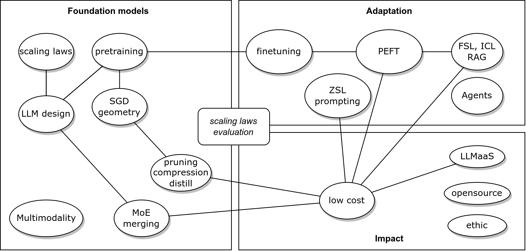
LLM: as a user
- Solving a task with LLMs:
- Download pretrained LLMs
- Adapt to a task
- Merge, compress them
- deploy, integrate (agents)
- Evaluate
LLM: as a designer
- Building an LLM:
- Design LLM architecture
- Gather, preprocess data
- Design training algos, toolings
- Track training, evaluate
- Release
- Our ambition today:
- Lay out fundamental blocks (attention, prompting, training…)
- Give insights (properties, where do they come from… )
- Tutorial oriented towards future practices (agents…)
Attention
- Intuition: transform word emb. using related context words
- See Lilian Weng blog

| Year | Authors | Contribution |
|---|---|---|
| 2014 | Graves et al | attention for Neural Turing Machines |
| 2014 | Bahdanau attention | application to NLP |
| 2015 | Luong attention | application to NLP |
| 2015 | Xu et al. | soft/global & hard/local |
| 2016 | Cheng, Dong and Lapata | self-att LSTMN |
| 2017 | Vaswani et al. | transformer, 120k citations |
KQV translation
\[\begin{equation} {\scriptsize{ \alpha_i = \frac {\exp(\text{score}(q,k_i))} {\sum_j \exp(\text{score}(q,k_j))} }} \end{equation}\] \[\begin{equation} {\scriptsize{ v' = \sum_i \alpha_i v_i }} \end{equation}\]
Similarity score
| name | score | ref |
|---|---|---|
| content-based | cosine\((q,k)\) | Graves14 |
| additive | \(v^T \tanh (W[q,k])\) | Bahdanau15 |
| location-based | \(\alpha = \text{softmax}(Wq)\) | Luong15 |
| general | \(q^T W k\) | Luong15 |
| dot-product | \(q^T k\) | Luong15 |
| scaled \(\cdot\) | \(\frac {q^t k} {\sqrt{d}}\) | Vaswani17 |
Scaled dot-product?
- Assume input E[k]=0 var(k)=1 \[var(xy) = (var(x)+E[x]^2)(var(y)+E[y]^2) - E[x]^2E[y]^2\]
- \(k\) and \(q\) independent: \(E[kq]=E[k]E[q]=0\) \[var(k_i q_i) = (var(k_i)+E[k_i]^2)(var(q_i)+E[q_i]^2) - E[k_i]^2E[q_i]^2 = 1\]
- Output variance: \[var\left(\sum_i k_iq_i\right) = \sum_i var(k_iq_i) = d\]
Self-attention
- Cheng 2016: use same sentence both for K and Q
- Often represented by a heat map over the words of the sentence
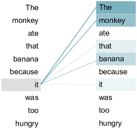
- Is attention interpretable? Does it enable explainability?
- No: cf. Why
Attentions May Not Be Interpretable?
- Combinatorial shortcuts: attention carry extra info for next layers
- Other approaches: Integrated gradients, SHAP…
Matrix formulation
- arrange all keys \(k_i\) as a
matrix \(K \in R^{N \times d}\)
- each vector \(k_i\) is a row of the matrix
- same for all queries \(q_i\) as \(Q \in R^{N \times d}\)
- \(A=\)sofmax\((QK^T)\)
- for each row, column, or globally?
- This matrix product outputs the new V = weighted sum of original V
- Beware of dimensions!
Self-attention with scaled dot-product:
\[V'=\text{softmax}\left(\frac {QK^T}{\sqrt{d}}\right)V\]
Cost
- The cost of \(QK^T\) is in \(O(n^2d)=O(n^2)\) operations
- But each of the \(n^2\) dot
products can be computed in parallel, so we have \(O(1)\) sequential operations
- Transformers are well adapted to GPU!
- Compare to RNN: \(O(n)\) sequential operations
from https://slds-lmu.github.io/seminar_nlp_ss20/attention-and-self-attention-for-nlp.html
| Layer | Complexity | Seq. op |
|---|---|---|
| recurrent | \(O(nd^2)\) | \(O(n)\) |
| conv | \(O(knd^2)\) | \(O(1)\) |
| transformer | \(O(n^2d)\) | \(O(1)\) |
| sparse transf | \(O(n\sqrt{n})\) | \(O(1)\) |
| reformer | \(O(n\log n)\) | \(O(\log (n))\) |
| linformer | \(O(n)\) | \(O(1)\) |
| linear transf. | \(O(n)\) | \(O(1)\) |
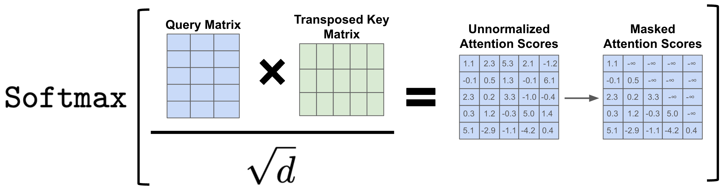
Training: Masked self-attention
- During training, the decoder is trained on sentence “The cat sat on
the mat”:
- Step 1: loss = \(p("The"|\emptyset)\)
- Step 2: loss = \(p("cat"|"The")\)
- Step 3: loss = \(p("sat"|"The cat")\) …
- This is causal LM
- We could give the decoder 6 sub-sentences (“The”, “The cat”, …)
- But it’s more efficient to give it the full sentence, and train with a causal mask:
Inference: KV cache
\[Q,K \in R^{N\times d}\] \[QK^T \in R^{N\times N}\]
- So storing \(QK^T\) requires \(O(n^2)\) memory
- A decoder (GPT) generates each token with auto-regression:
- Each step recomputes self-att with \(N \leftarrow N+1\)
- We are recomputing each time the same attentions!
- Solution: save the already computed \(K\) and \(V\):
KV cache
- KV cache leads to
- faster matrix computations
- more memory to store cache
- New enhancements:
- KV cache quantization
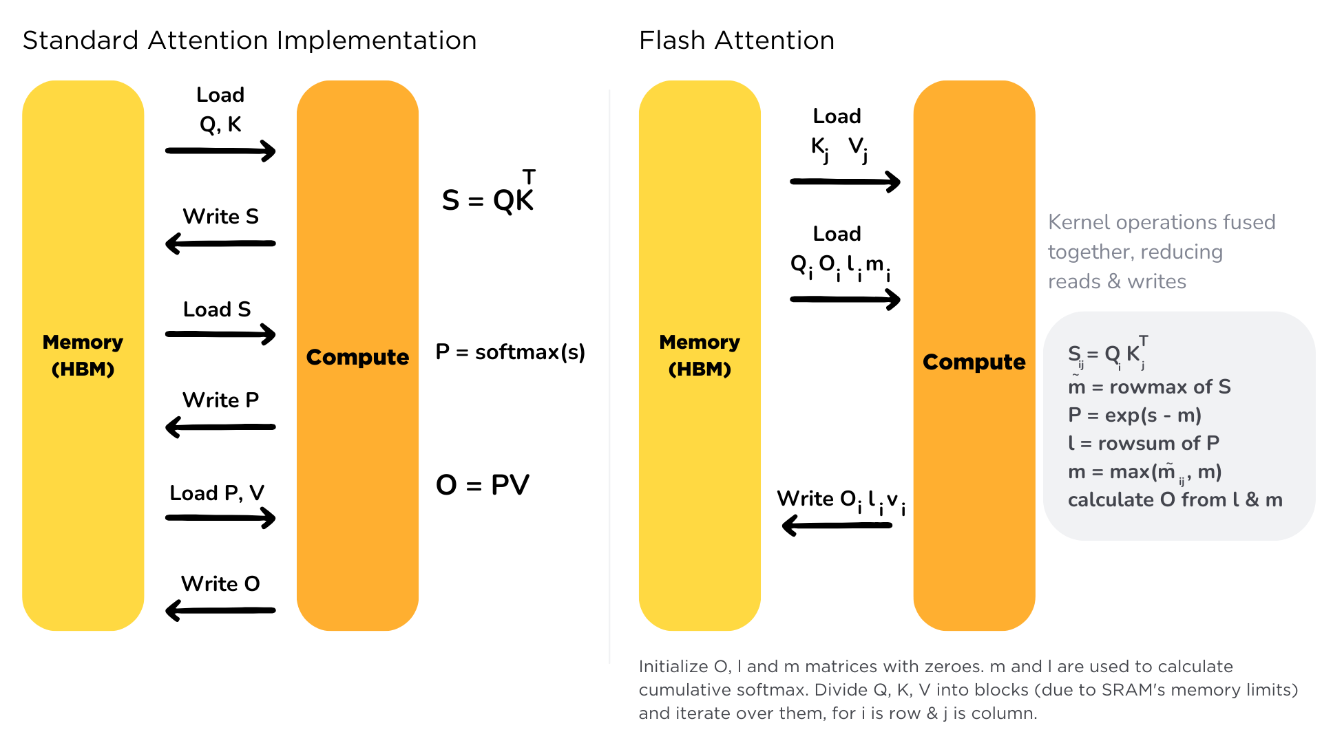
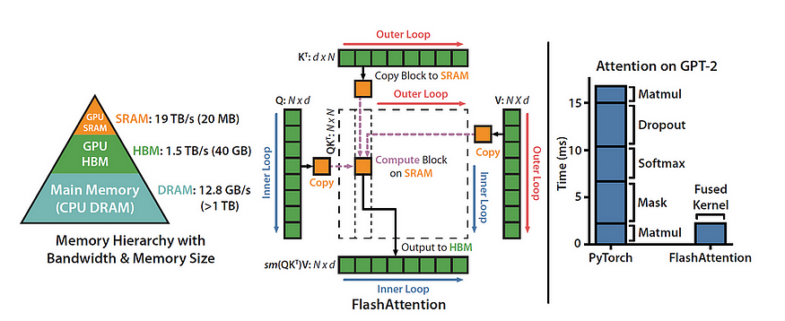
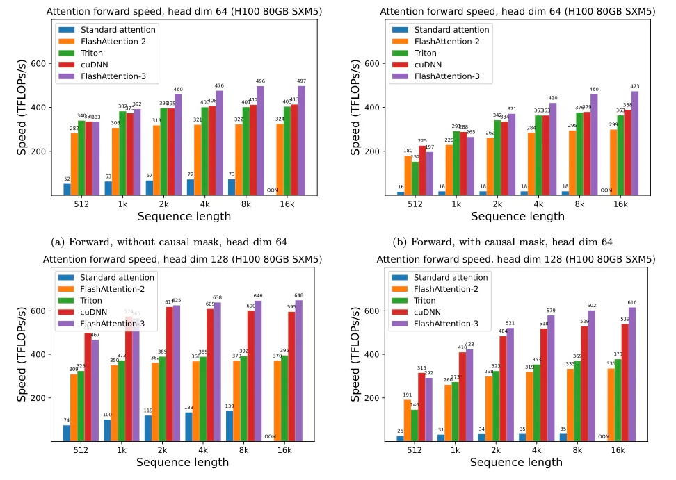
Flash Attention
- Bottleneck: memory I/O
- High Bandwidth Memory = large but slow
- GPU on-chip SRAM = small but fast
- Solution:
- fused kernels for self-att
- stay on-chip
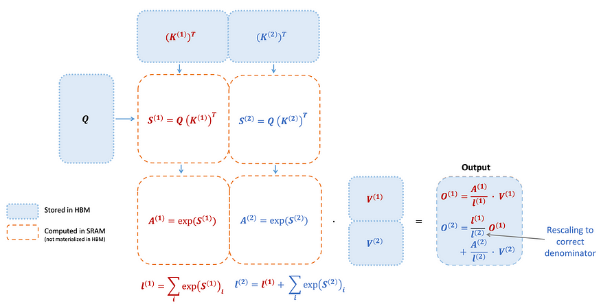
Flash Attention 2
- Divides and parallelizes the computation with the K and V matrices
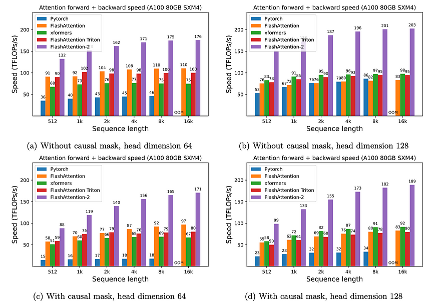
Flash Attention 3
- adapted to H100 GPU
- overlap warped matmuls and softmax
- FP8 “incoherent processing” (see QuiP) = multiplies the query and key with a random orthogonal matrix to “spread out” the outliers and reduce quantization error
Kernel optim on CPU
matmul on python: 0.042 GFLops
numpy (FORTRAN): 29 GFlops
reimplementation of numpy in C++: 47 GFlops
BLAS with multithreading: 85 GFlops
llama.cpp (focus matrix-vec): 233 GFlops
Intel’s MKL (closed source): 384 GFlops
OpenMP(512x512 matrix): 810 GFlops
exported in llamafile: 790 GFlops
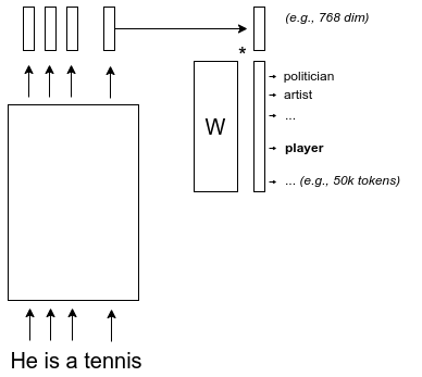
Transformer
(Vaswany et al., Google, 2017)
![]()
Details of the stack
- Bottom:
- convert input tokens to static embedding vectors \(X_t\)
- table lookup in Embeddings matrix
- Embeddings trained along with all other parameters (\(\neq\) contrastive)
- 3 matrices transform input embeddings \(X\) into \(Q,K,V\)
- convert input tokens to static embedding vectors \(X_t\)
Positional Encodings
- Self-attention gives the same repr when you shuffle the words !
- Inject information about position through a vector that encodes the position of each word
- Naive approaches:
- \(p=1,\dots,N\): not normalized + never seen N
- \(p=0,0.06,\dots,1\): \(\Delta p\) depends on sentence length
- Better approach:
- inspired by spectral analysis
- positions are encoded along sinusoidal cycles of various frequencies
\[p_t^{(i)} = \begin{cases} sin(w_k \cdot t), \text{if }i=2k \\ cos(w_k \cdot t), \text{if }i=2k+1 \end{cases}\]
with \(d\) encoding dim and
\[w_k = \frac 1 {10000^{2k/d}}\]
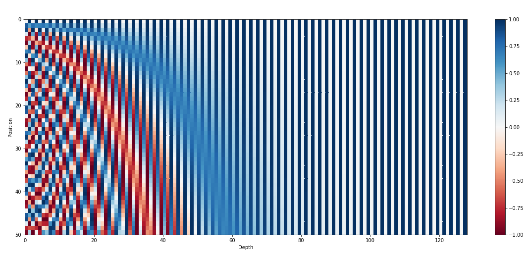
- Remarks:
- by giving positional encodings the same dimension as word embeddings, we can sum them together
- most positional information is encoded in the first dimensions, so summing them with word embeddings enable the model to “let” the first dimensions free of semantics and dedicate them to positions.
- Challenge: long-context
Multi-head self-attention
- several attentions in parallel
- concat outputs after self-att
![]()
Normalisation
- Add a normalization after self-attention
- parametric center+scale 1 vec across dimensions
- keep gradients small (cf arxiv.org/pdf/2002.04745)
MLP = feed forward
- Add another MLP to store/inject knowledge
- Add residual connections: smooth loss landscape
Layer
- Stack this block \(N\) times
- Gives time to reason = execution steps of a program
- Enables redundancy: Mechanistic interpretability:
- developped by Anthropic AI
- multiple/concurrent circuits
Encoder-decoder
- The transformer is designed for Seq2Seq
- So it contains both an encoder and decoder
- Same approach for decoder
- with cross-attention from encoder to decoder matching layers
- with masks to prevent decoder from looking at words \(t+1, t+2\dots\) when predicting \(t\)
- GPT family: only the decoder stack
- BERT family: only the encoder stack (+ classifier on top)
- T5, BART family: enc-dec
- pure encoders (BERT) have been superseded by enc-dec (T5)
- because T5 learns multiple tasks at once, vs. 1 task for BERT
- advantage of denoising loss decreases with scale
- denoising loss are less efficient than next-token prediction => largest LLMs are all encoders
- Implementation details of the transformer:
- great resource:
- see The annotated transformer
Inductive bias of transformer
- Assume discrete inputs (tokens)
- All positions in sentence have equal importance
- Relates tokens based on similarities / content
- 2 major composants with different roles:
- self-att focuses on relations
- MLP inject knowledge
- Solve limitations of previous models
- No bottleneck of information (as in ConvNet, RNN, seq2seq…)
- No preference for “recent tokens” (as in RNN)
- No constraints of locality (as in CNN)
- after learning, transformer can be viewed as a semi-Turing Machine:
- proof that it applies gradient descent, each layer = 1 step
- another proof that it can apply temporal difference (RL algo)
- conclusion: it learns algorithms
- see also Information Bottleneck
Desirable properties
- Can scale (cf. scaling laws)
- Can “absorb” information: the web on a USB stick
- Can “compress” information
- 2 dims to reason: time + layers
- Support all modalities
- Language transformers: a central place
- “Absorb” the written web == all human knowledge
- by far the largest transformers
- 2021: Wu Dao 2.0: 1.75 trillion parameters
- Other modalities enrich LLM
Terminology
- Activations: output of each layer
- Embeddings: outputs of the embeddings layer
- Latent representations: all activations
- LM head: final linear layer that outputs 1 score/voc unit
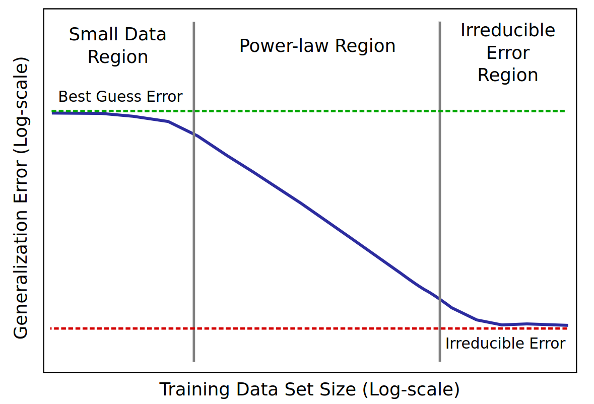
Scaling laws
Chinchilla law

Scaling LLMs
- The more data you train on
- the more the LLM knows about
- the better the LLM generalizes
- scaling law = power law = \(y(x) = ax^{-\gamma} +b\)
- \(y(x) =\) test loss
- \(\gamma\) = slope
Baidu paper 2017
Scaling laws for Neural LM 2020
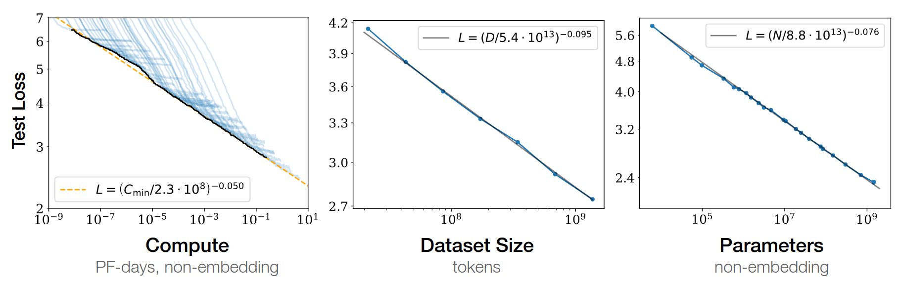
Open-AI 2020
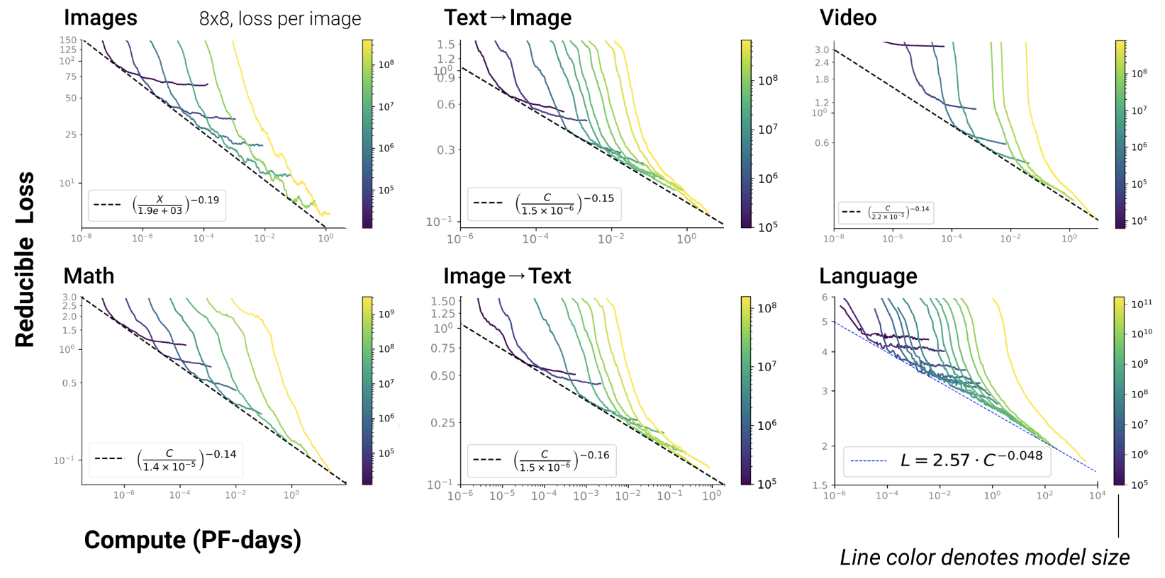
- RL, protein, chemistry…
Chinchilla paper 2022
- GPT3 2020: inc. model capacity
- Chinchilla 2022: inc. data

\(L=\) pretraining loss


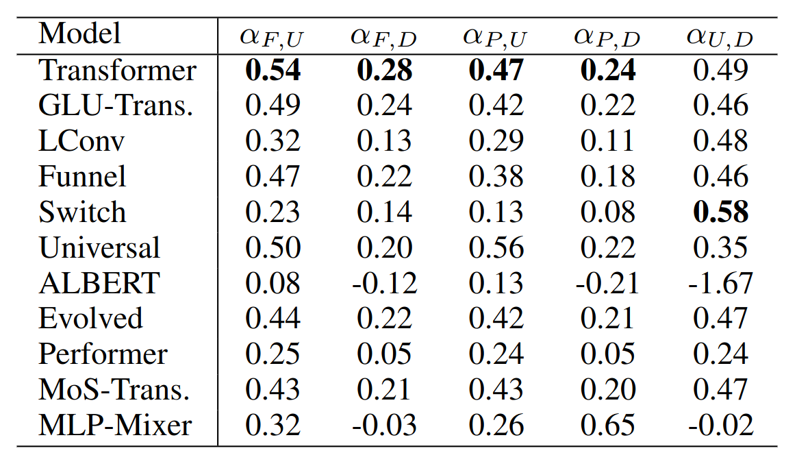
Google 2022: paper1, paper2 Flops, Upstream (pretraining), Downstream (acc on 17 tasks), Params
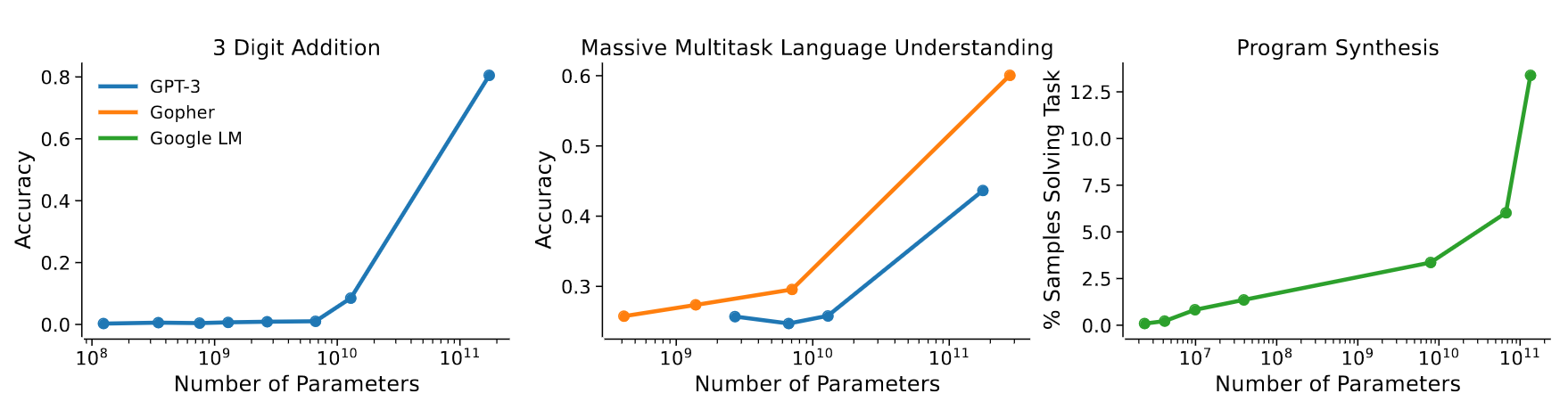
Emerging capabilities
- Scaling laws exist in Machine Learning for a long time (cf. Paper on learning curves)
- But it’s the first time they result from emerging capabilities!
GPT3 paper 2020
- emergence of “In-Context Learning”
- = capacity to generalize the examples in the prompt
- example:
"manger" devient "mangera"
"parler" devient "parlera"
"voter" devient
Anthropic paper 2022
- shows that the scaling law results from combination of emerging capabilities
Jason Wei has exhibited 137 emerging capabilities:

- In-Context Learning, Chain-of-thought prompting
- PoT, AoT, Analogical prompting
- procedural instructions, anagrams
- modular arithmetics, simple maths problems
- logical deduction, analytical deduction
- physical intuition, theory of mind ?
- …
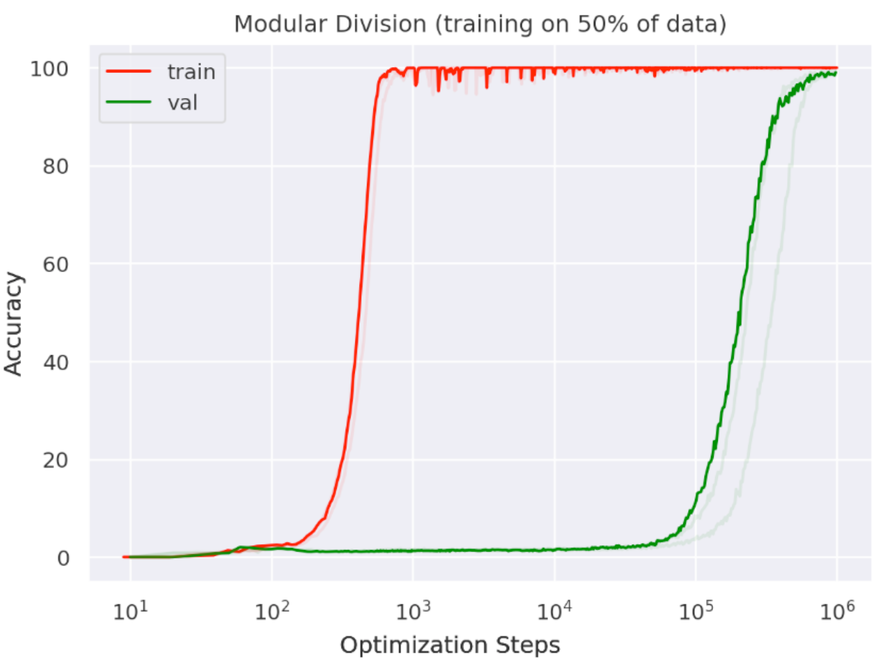
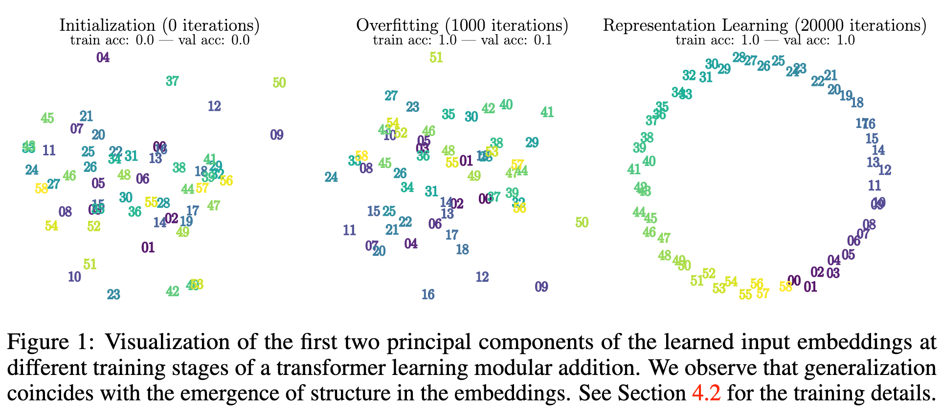
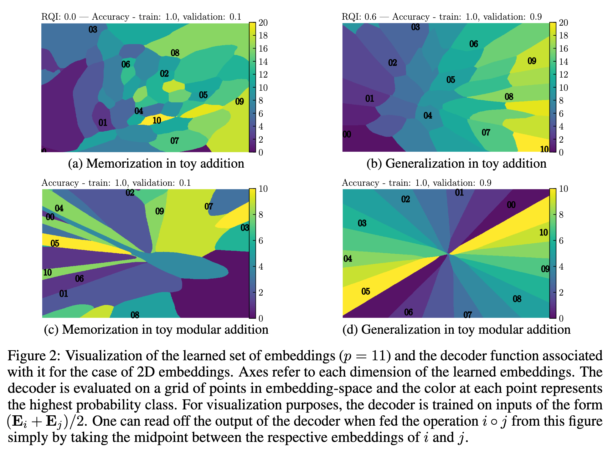
LLM structure information
During training, they may abruptly reorganize their latent representation space
LLM
Life cycle of LLM

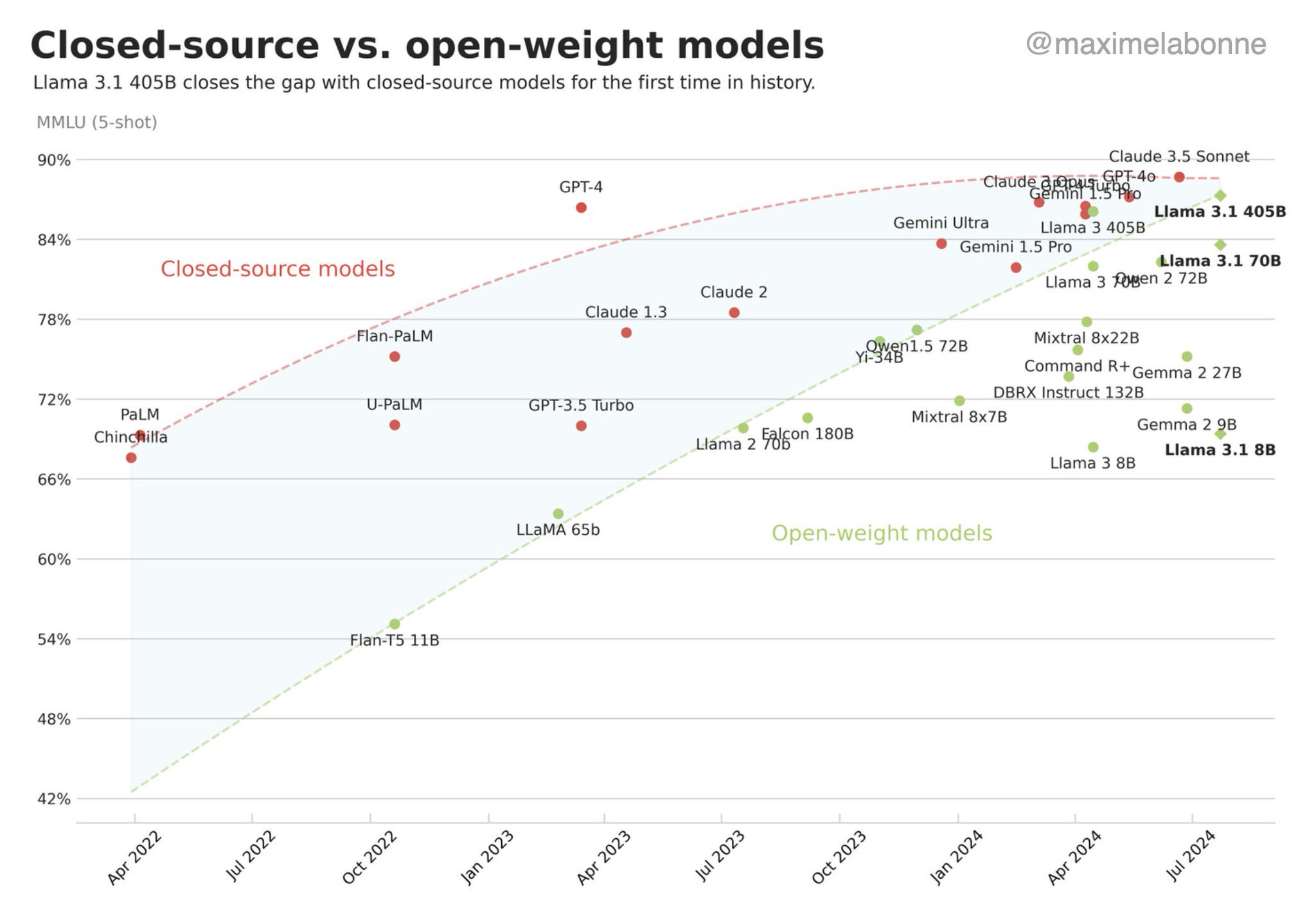
Open-source community
- Extremely important for LLMs:
- “We have no moat” (Google, 2023)
- Main contributors in: pretraining, finetuning, model merging, dissemination, efficiency, evaluation
- Main open-source actors:
- Companies: Meta, HuggingFace, Eleuther AI, Mistral, Together AI, Cerebras…
- Civil society: passionates, geeks (TheBloke, Teknium…)
- Academics
- Online: Huggingface-hub, discord
- Towards specialization:
- Foundation: Meta, Eleuther, Mistral…
- Prompting: CoT, PoT, AoT…
- Finetuning: 1M models on HF
- Integrators: LangChain, DSPy, Coala…
- Academics: theory, app domains…
- Conversely to code, there’s a continuum between “fully open” and
“closed” source:
- distribute model weights
- distribute code
- distribute training logs
- distribute training data
- …
LLM and AI-Act

New research fields
- For now: empirical science; observations:
- memorisation, compression, structuration, generalisation
- grokking, emerging capacities
- Embryos of theories:
- Chinchilla scaling laws
- grokking: circuits
- double descent, geometry of the loss
- phase transitions, singularity…
Pretraining
- Most important step:
- store all knowledge into the LLM
- develop emergent capabilities
- Most difficult step
Principle:
- Train model on very large textual datasets
- ThePile
- C4
- RefinedWeb
- …
Training
- Next token prediction
Training algorithm: SGD
- Initialize parameters \(\theta\) of LLM \(f_\theta()\)
- Stochastic Gradient Descent:
- Sample 1 training example \((x_{1\dots T-1},y_T)\)
- Compute predicted token \(\hat y_T = f_\theta(x_{1\dots T-1})\)
- Compute cross-entropy loss \(l(\hat y_T, y_T)\)
- Compute gradient \(\nabla_\theta l(\hat y_T, y_T)\)
- Update \(\theta' \leftarrow \theta -\epsilon \nabla_\theta l(\hat y_T, y_T)\)
- Iterate with next training sample
Compute gradient: back-propagation
- Compute final gradient \(\frac{\partial l(\hat y_T, y_T)}{\partial \theta_{L}}\)
- Iterate backward:
- Given “output” gradient \(\frac{\partial l(\hat y_T, y_T)}{\partial \theta_{i+1}}\)
- Compute “input” gradient: \(\frac{\partial l(\hat y_T, y_T)}{\partial \theta_{i}} = \frac{\partial l(\hat y_T, y_T)}{\partial \theta_{i+1}} \frac{\partial \theta_{i+1}}{\partial \theta_i}\)
- every operator in pytorch/tensorflow is equipped with its local derivative \(\frac{\partial \theta_{i+1}}{\partial \theta_i}\)
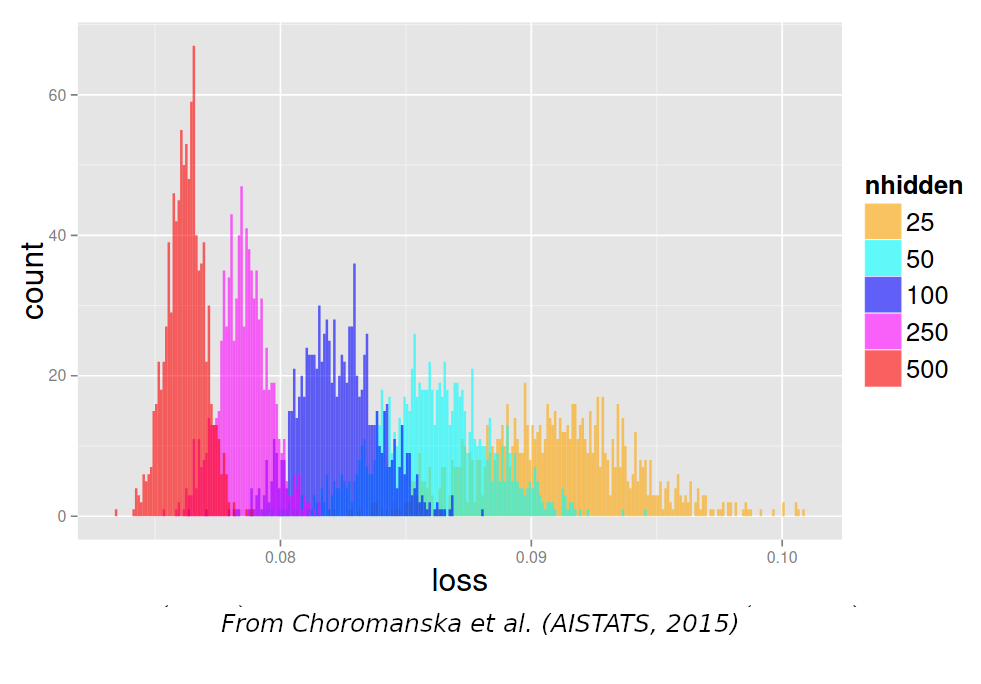
Local optima
- Proof that SGD converges to a local optimum
- All local minima are global: Kawaguchi,2019
Key ingredients to success:
- The prediction task is forcing the model to learn every linguistic level
- The model must be able to attend long sequences
- Impossible with ngrams
- The model must have enough parameters
- Impossible without modern hardware
- The model must support a wide range of functions
- Impossible before neural networks
- The data source must be huge
LLMs store knowledge
- “Give me a recipe to cook bacon”
- “place the bacon in a large skillet and cook over medium heat until crisp.”
- “The main characters in Shakespeare’s play Richard III are”
- “Richard of Gloucester, his brother Edward, and his nephew, John of Gaunt”
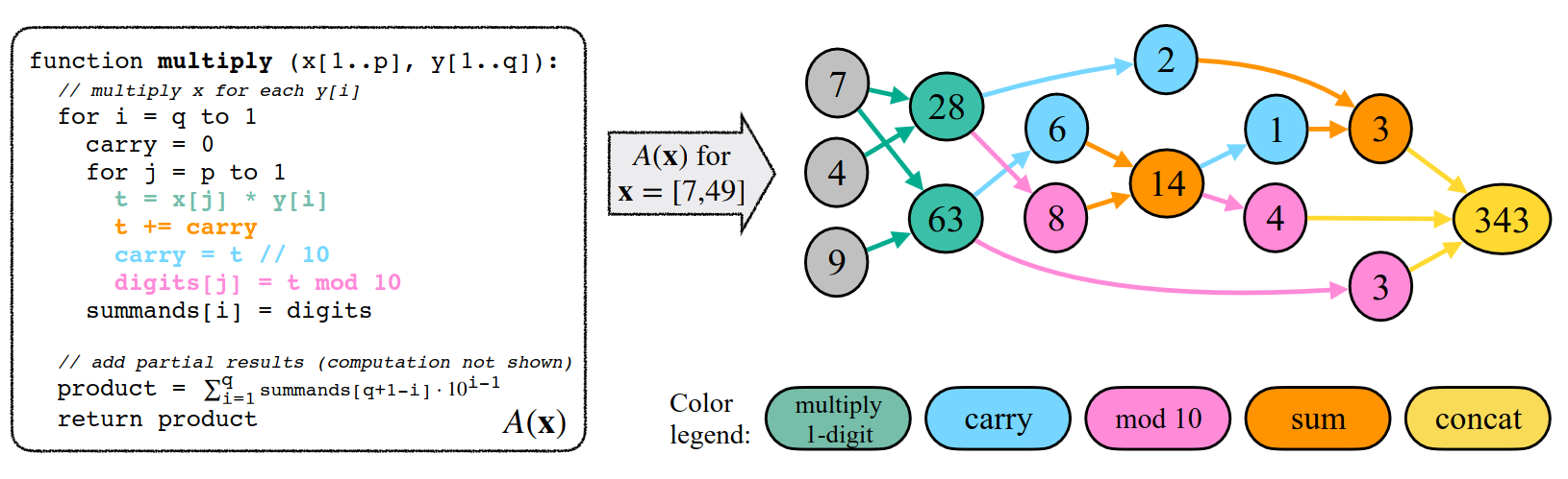
LLMs “reason”
- “On a shelf, there are five books: a gray book, a red book, a purple
book, a blue book, and a black book. The red book is to the right of the
gray book. The black book is to the left of the blue book. The blue book
is to the left of the gray book. The purple book is the second from the
right. Which book is the leftmost book?”
- “The black book”
- Reasoning of an LLM:
- Remember algorithms that generate training samples
- Match/combine subgraphs
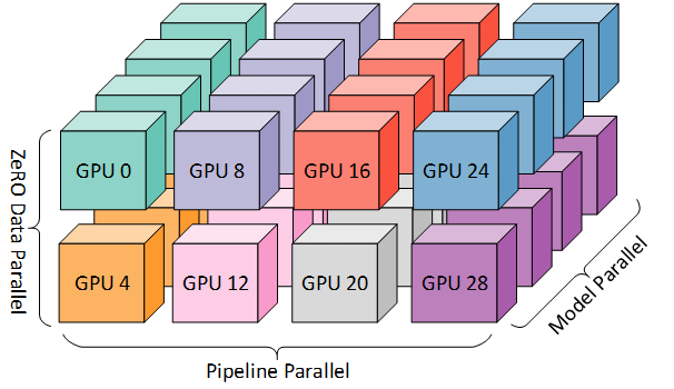
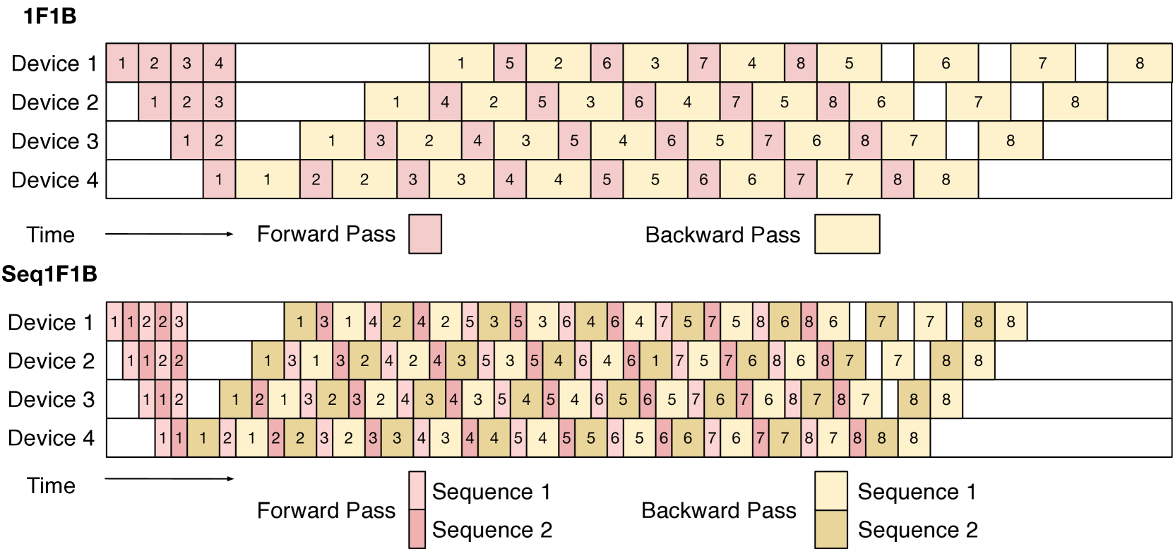
Training at scale
Data P., model sharding, Tensor P., Sequence P., pipeline P…
- Tooling:
- Megatron-DS
- Deep Speed
- Accelerate
- Axolotl
- Llama-factory
- …
Mixtral, Mamba, Llama-3.1
Choice of architecture
- Focus on representations: RAG, multimodal,
recommendation
- contrastive learning: S-BERT, BGE, E5
- Focus on generation:
- Transformer-based LM
- MoE
- SSM: S4, Mamba
- Diffusion
Mixture of Experts
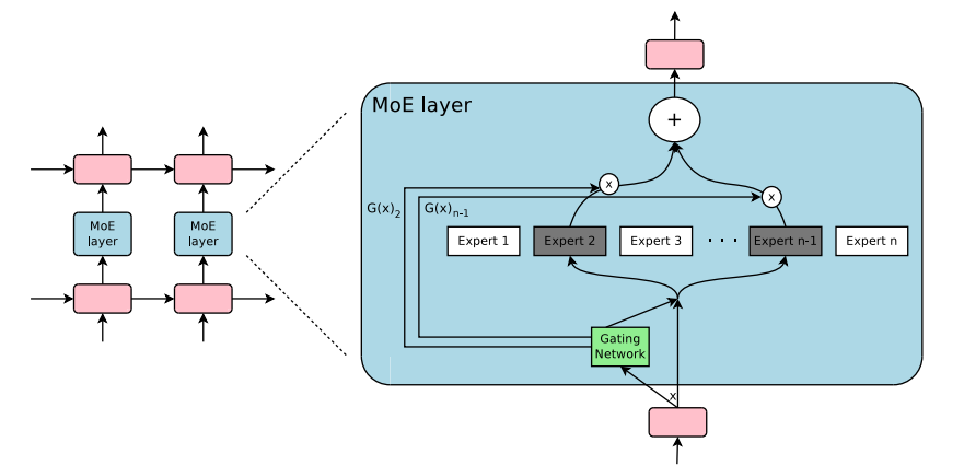
(from huggingface)
Mixture of Experts
- Main advantage: reduced cost
- Ex: 24GB VRAM (4-bit Mixtral-8x7b) 7b-params during forward pass
- Drawbacks:
- more redundancy across parameters
- hard to train
State-Space Models
- Discrete SSM equation similar to RNN:
\[h_t = Ah_{t-1} + Bx_t\] \[y_t = Ch_t + D x_t\]
- but A,B,C,D are computed: they depend on the context
Mamba
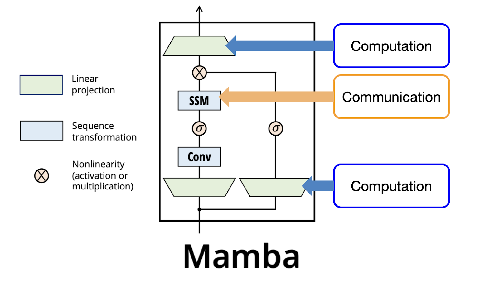
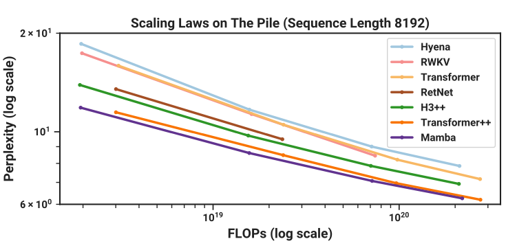
- scaling law comparable to transformer (up to \(10^{20}\) FLOPs)
- linear \(O(n)\) in context length
- faster inference, but slower training
Diffusion transformer
- Diffusion models: forward noise addition
- Adds noise, step by step to input \[q(x_t|x_{t-1}) = N(x_t;\sqrt{1-\beta_t} x_{t-1}, \beta_t I)\]
- backward denoising process
- starts from white noise
- reverse the forward process with a model (U-Net or transformer): \[p_\theta(x_{t-1}|x_t) = N(x_{t-1}, \mu_\theta(x_t,t), \Sigma_\theta(x_t,t))\]
- iteratively denoise
Many text diffusion models

(from PMC24)
Comparison
- Diffusion models are much slower than LLM, because of many sampling steps
- But they produce a complete sentence at each step
Number of parameters
- Assume a transformer is chosen. How many parameters should it have?
- What is the main constraint?
- Training compute
- Inference/deployment compute
- What is the main constraint?
- When the LLM must be deployed on limited hardware, choose a small size and train it as long as possible
- Let’s study the case of Llama3.1:
- Main constraint = training compute = \(3.8\times 10^{25}\) FLOPs
- Chinchilla scaling laws not precise enough at that scale, and not for end-task accuracy
- so they recompute they own scaling laws on ARC challenge benchmark!
- They fix compute \(c\) (from \(10^{18}\) a \(10^{22}\) FLOPs)
- They pick a model size \(s\), deduce from \((s,c)\) the nb of data points \(d\) the model can be trained on
- They train it, get the dev loss \(l(s,c,d)\)
- They plot the point \((x=d,y=l)\)
and iterate for a few other \(s\)
- For each \(c\), they get a quadratic curve: why?
- Because:
- the largest model is more costly to train, so it’s trained on the fewest data (\(x_{min}\))
- when it’s too large, it’s trained on too few data \(\rightarrow\) high loss
- the smallest model is trained on lots of data (\(x_{max}\))
- but it has too few parameters to memorize information \(\rightarrow\) high loss
- so there’s a best compromise in between
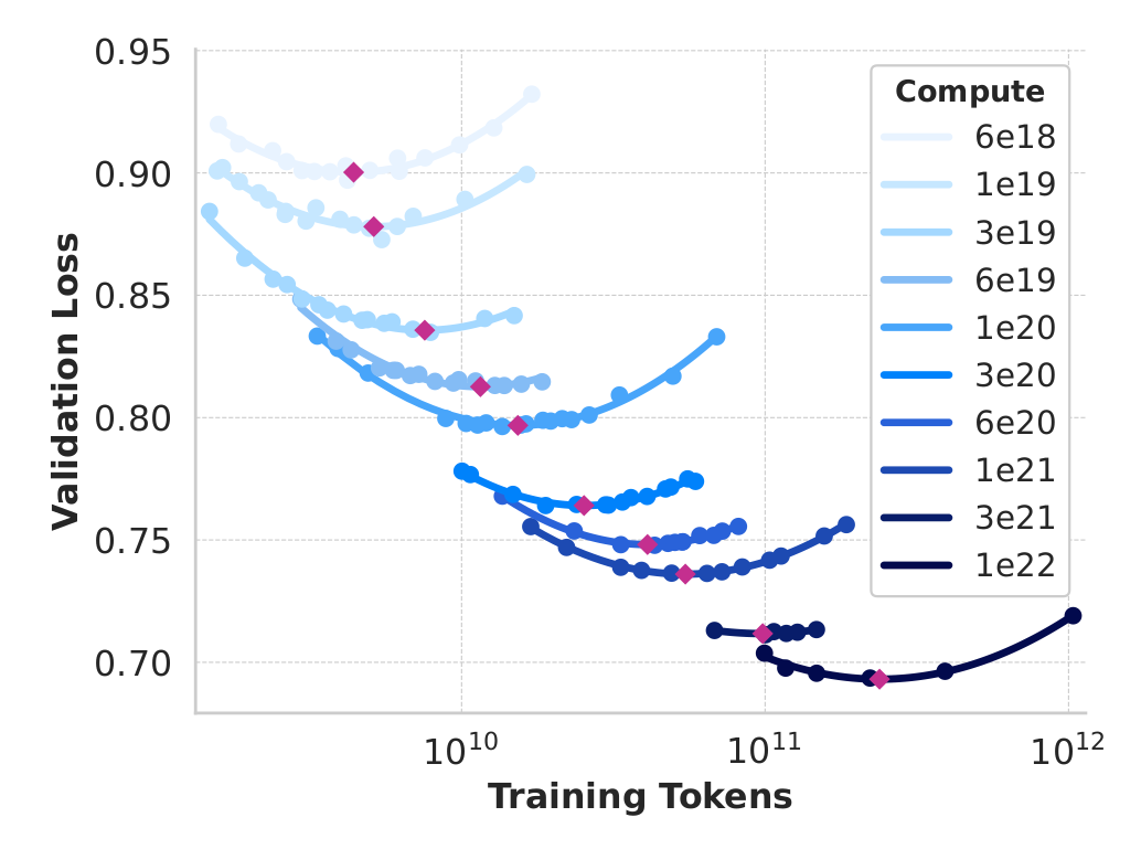
- Terminology:
- compute = nb of operations to train
- IsoFLOP curve = plot obtained at a constant compute
- compute-optimal model = minimum of an IsoFLOP curve
- But these scaling laws are mostly computed at “low” FLOPs range
- So they compute for these models & the largest llama2 models both the dev loss and accuracy
- They assume a sigmoid relation btw loss & accuracy
- They extrapolate the scaling law with this relation, and get 405b parameters
Local usage
- With Zero-Shot learning
- With few-shot learning
- As frozen embeddings
- With fine-tuning
- With prompt tuning
- With Zero-label Unsupervised Data Generation
- …
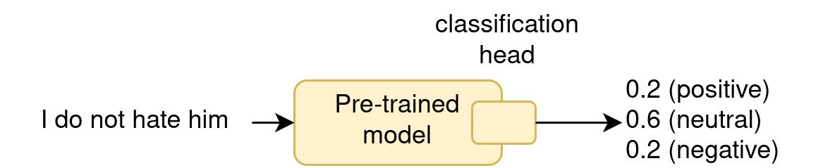
Zero-Shot Learning
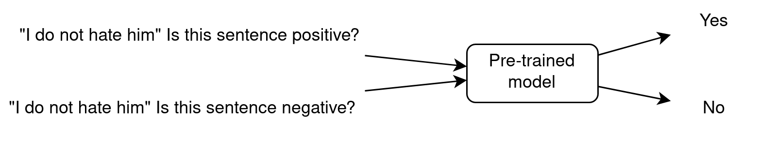
- Zero-Shot because the LLM has been trained on task A (next word prediction) and is used on task B (sentiment analysis) without showing it any example.
In-context Few-Shot Learning
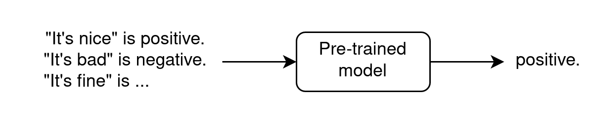
- requires very few annotated data
- In context because examples are shown as input
- does not modify parameters
- see paper “Towards Zero-Label Language Learning” (GoogleAI, sep 2021)
As frozen embeddings
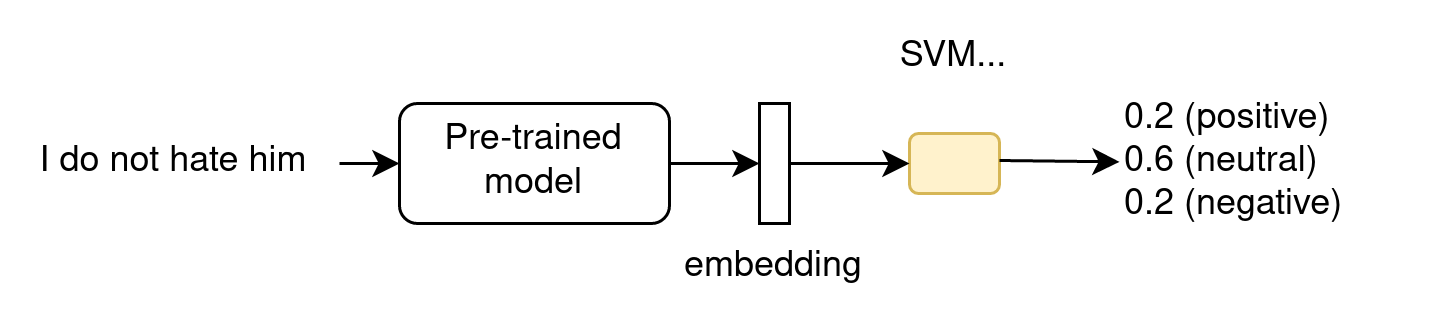
- does not modify the LLM parameters
- for ML-devs, as the LLM is part of a larger ML architecture
With fine-tuning
- does modify the LLM parameters !
- often give the best results
- Difference between finetuning and continued pretraining (continual
learning, CL):
- FT: adapt the LLM to a domain, a language, a task…
- FT: the LLM will loose other capacities
- CL: inject new knowledge into the LLM
- CL: capture the language drift
- CL: the LLM stays generic, and can still be FT on many tasks
With Parameter-efficient tuning (PEFT)
See course on Wednesday afternoon!
Zero-label Unsupervised Data Generation
- Generate synthetic samples with few-shot; e.g., prompt=
- task description
- samples
- ask to generate samples for a given label
- Finetune a model on this dataset
Prompt engineering
Workflow:
- define tasks
- write prompts
- test prompts
- evaluate results
- refine prompts; iterate from step 3
Template of prompt
<OBJECTIVE_AND_PERSONA>
You are a [insert a persona, such as a "math teacher" or "automotive expert"]. Your task is to...
</OBJECTIVE_AND_PERSONA>

<INSTRUCTIONS>
To complete the task, you need to follow these steps:
1.
2.
...
</INSTRUCTIONS>

------------- Optional Components ------------

<CONSTRAINTS>
Dos and don'ts for the following aspects
1. Dos
2. Don'ts
</CONSTRAINTS>

<CONTEXT>
The provided context
</CONTEXT>

<OUTPUT_FORMAT>
The output format must be
1.
2.
...
</OUTPUT_FORMAT>

<FEW_SHOT_EXAMPLES>
Here we provide some examples:
1. Example #1
  Input:
  Thoughts:
  Output:
...
</FEW_SHOT_EXAMPLES>

<RECAP>
Re-emphasize the key aspects of the prompt, especially the constraints, output format, etc.
</RECAP>
Notes
- few-shot examples are mainly used to define the format, not the content!
- attribute a role that is relevant for the task
- use prefixes for simple prompts:
TASK:
Classify the OBJECTS.

CLASSES:
- Large
- Small
OBJECTS:
- Rhino
- Mouse
- Snail
- Elephant- use XML or JSON for complex prompts
Ask for explanations
What is the most likely interpretation of this sentence? Explain your reasoning. The sentence: “The chef seasoned the chicken and put it in the oven because it looked pale.”
- Llama3.1-7b: “[…] the chef thought the chicken was undercooked or not yet fully cooked due to its pale appearance […]”
CoT for complex tasks
Extract the main issues and sentiments from the customer feedback on our telecom services.
Focus on comments related to service disruptions, billing issues, and customer support interactions.
Please format the output into a list with each issue/sentiment in a sentence, separated by semicolon.

Input: CUSTOMER_FEEDBACK
Classify the extracted issues into categories such as service reliability, pricing concerns, customer support quality, and others.
Please organize the output into JSON format with each issue as the key, and category as the value.
Input: TASK_1_RESPONSEGenerate detailed recommendations for each category of issues identified from the feedback.
Suggest specific actions to address service reliability, improving customer support, and adjusting pricing models, if necessary.
Please organize the output into a JSON format with each category as the key, and recommendation as the value.
Input: TASK_2_RESPONSECoT workflow
- break the pb into steps
- find good prompt for each step in isolation
- tweak the steps to work well together
- enhance with finetuning:
- generate synthetic samples to tune each step
- finetune small LLMs on these samples
Alternative: DSPy
- optimize prompts automatically
- you define the target metric
- DSPy uses LM-driven optimizers to tune prompts and weights
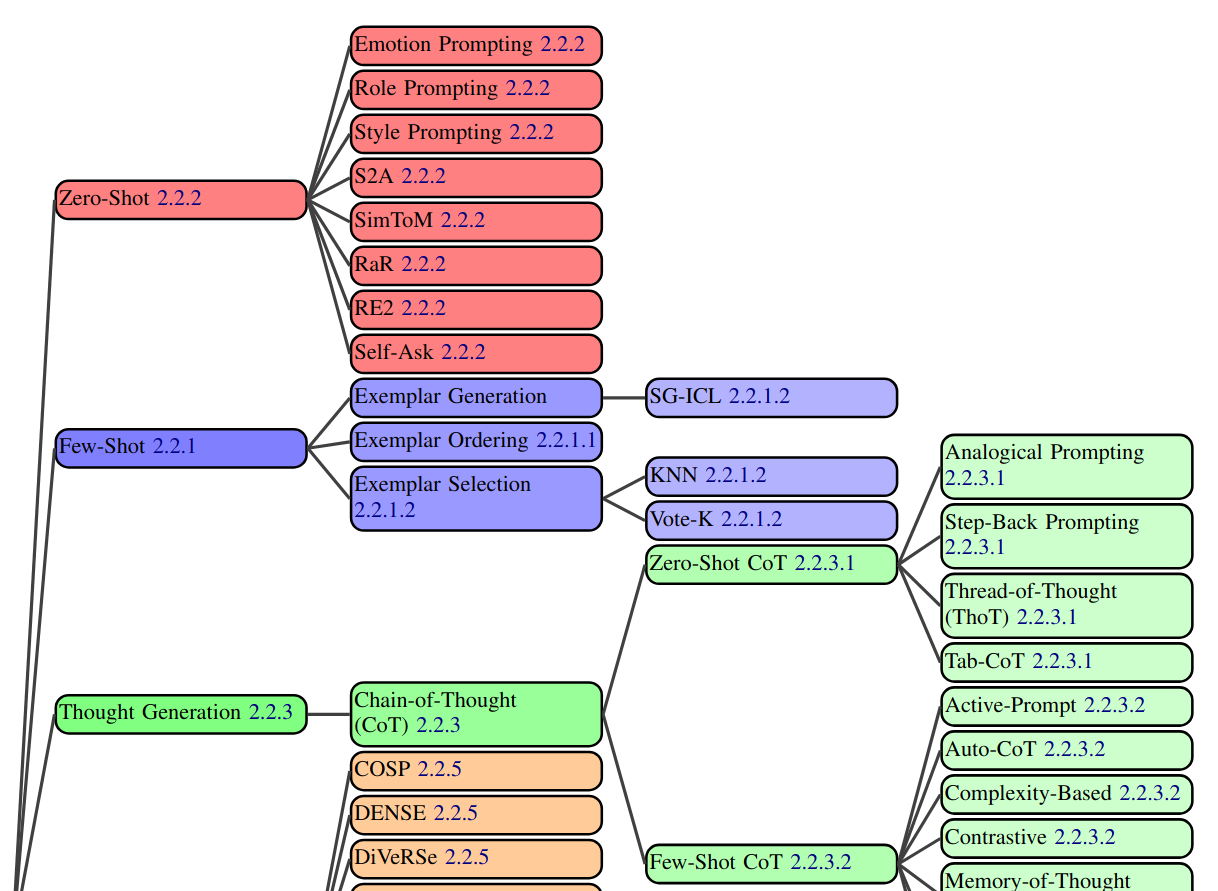
- Vanilla prompting
- Chain-of-thought (CoT)
- Self-consistency
- Ensemble refinment
- Automatic chain-of-thought (Auto-CoT)
- Complex CoT
- Program-of-thoughts (PoT)
- Least-to-Most
- Chain-of-Symbols (CoS)
- Structured Chain-of-Thought (SCoT)
- Plan-and-solve (PS)
- MathPrompter
- Contrastive CoT/Contrastive self-consistency
- Federated Same/Different Parameter self-consistency/CoT
- Analogical reasoning
- Synthetic prompting
- Tree-of-toughts (ToT)
- Logical Thoughts (LoT)
- Maieutic Prompting
- Verify-and-edit
- Reason + Act (ReACT)
- Active-Prompt
- Thread-of-thought (ThOT)
- Implicit RAG
- System 2 Attention (S2A)
- Instructed prompting
- Chain-of-Verification (CoVe)
- Chain-of-Knowledge (CoK)
- Chain-of-Code (CoC)
- Program-Aided Language Models (PAL)
- Binder
- Dater
- Chain-of-Table
- Decomposed Prompting (DeComp)
- Three-Hop reasoning (THOR)
- Metacognitive Prompting (MP)
- Chain-of-Event (CoE)
- Basic with Term definitions
- Basic + annotation guideline + error-analysis- lists the best prompting techniques for every possible NLP task.
- Another survey of prompt engineering
Examples of prompts
Practical session
- Local LLM server with ollama
- Tools use: make the LLM aware of the latest news