LLM
Christophe Cerisara
2024/2025
LLM: introduction
- dates: check monade.univ-lorraine.fr!
| CM |
|---|
| 03/09 |
| 05/09 |
| 12/09 |
| 19/09 |
| 26/09 |
| 03/10 |
| 10/10 |
| 28/11 |
| 05/12 |
| 12/12 |
| 27/01 |
| Topic | |
|---|---|
| LLM fundamentals | embeddings, ranking loss |
| attention | |
| transformer | |
| properties | scaling laws, emergence |
| usage, adaptation | local usage: ZSL, FSL, ICT, FT |
| PEFT | |
| training | pretraining |
| transforming | compression, pruning, distillation, merging |
| mastering | best practices |
Every topic
- course
- practice
- MCQ
Course requirements:
- Basics of python
- Access to a computer (in & outside class)
- With python + pytorch + transformers installed
- Internet access in & outside class (eduroam)
- Any question:
- cerisara@loria.fr
- slides: https://members.loria.fr/CCerisara/#courses/llm/
LLM concepts
Objectives and design
- Why using an LLM?
- Bring world knowledge & reasoning
- Manipulate natural languages
- generic tools
- But for specific data/task
- xgboost is better
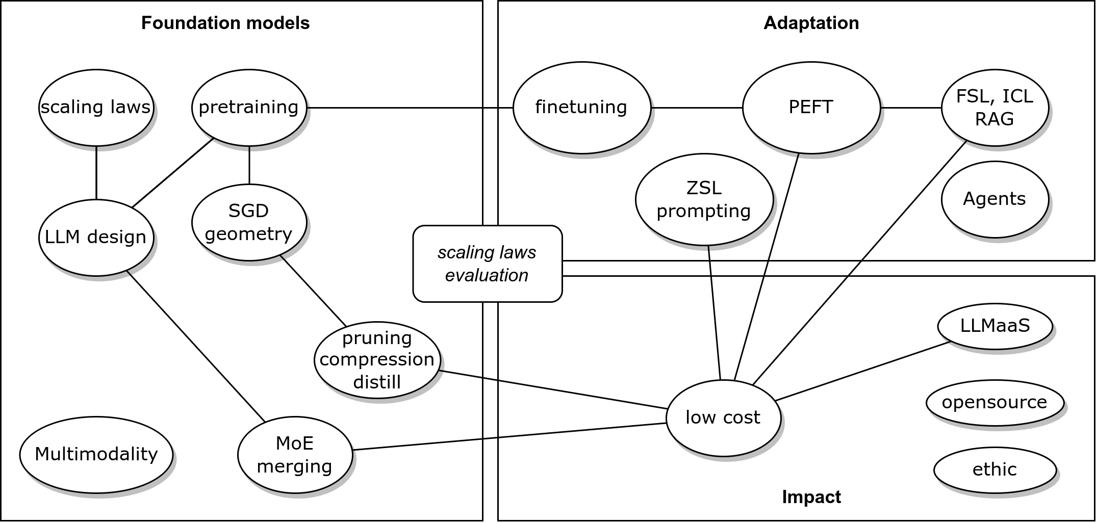
Choice of LLM
- Want to solve a task:
- Download pretrained LLMs
- Adapt to a task
- Merge, compress them
- deploy, integrate (agents)
- Evaluate
- Want to build LLM:
- Design LLM architecture
- Gather, preprocess data
- Design training algos, toolings
- Track training, evaluate
- Release
- Recent architectures
- Focus on representations: embeddings
- Focus on generation:
- Transformer-based LM
- MoE
- SSM: S4, Mamba
- Diffusion
Content of today’s course
- Concepts of embeddings
- History and evolution of embeddings
- Training embeddings
- Controlling the embeddings space: contrastive loss
- Embeddings and RAG
- Tokenization
Importance of embeddings
- Embedding = representation of input into a vector space
- Input = words (BERT), sentences (SBERT, E5, BGE), captioned images (CLIP)…
- Used for:
- retrieval (RAG)
- multimodal models
One-hot encoding
- Orthogonal normed vectors: all words are equal
- Can be processed with matrix algebra
- But high dim and fixed vocabulary
- highly sub-optimal (symetries)
Word embedding
- Goal: low-dim vectors separated by semantics distances
Cosine similarity: \(sim(w,u)=\frac {u \cdot v}{||u||~~||v||}\)
Training word embeddings
- How to build a semantic embedding space?
- Using distributional hypothesis: “You shall know a word by the company it keeps” [Firth, 1957]
- Implementations:
- Probabilistic Models
- Vector Space Models
- Neural embeddings
Probabilistic models
- Blei, Ng and Jordan, 2003
- Latent Dirichlet Allocation: learn the distributions
- P(word | topic) and P(topic | document)
- P(topic | document) == document embedding
- Can infer P(topic | word) == (explainable) word embedding!
Vector space models
- Word embedding = vector of nb of occurrences of word in each
document
- == term-document matrix
- But high dim, noisy
- Methods to “compress” the matrix:
- Latent Semantic Analysis (LSA) (1990), HAL (1997), BEAGLE (2007), Glove (2014)
- Special case: random indexing (2006)
Random indexing
Johnson-Lindenstrauss lemma: projection into random high-dim subspace approx. preserves distances
Init: each word \(w\) is assigned an index random sparse vector \(I_w\), and a context null vector \(C_w\).
For every \(u\) in the context of \(w\): \(C_w \leftarrow C_w + I_u\)
Very fast
Incremental
Neural static embeddings
- “word embedding” proposed by Bengio in 2003
- Collobert embeddings (2008): trained on NLP tasks
- Word-to-vec (Mikolov, 2013): trained to predict context
- Problems: OOV? Polysemy? MWE?…
Contextual embeddings
- Recompute an embedding for every context
- “The XLS table” vs. “The cat sat on the table”
- ELMo: char-based, LM training, bi-dir RNN
- BERT: subwords, Masked-LM training, transformer (encoder)
- GPT: BPE, LM training, transformer (decoder)
- XLNet: improved BERT, permutation-LM training, transformer-XL
Sentence embeddings
- NN-LM (Bengio): \(s = P(w_t|w_1,\dots,w_{t-1})\)
- Averaging word embeddings: \(s=\frac 1 T \sum_t w_t\)
- Doc2Vec (Mikolov): Avg with paragraph vector
- Skip-thought: generates context sentences
- Quick-thought: classifies candidates context sentences
- InferSent: trained on NLI
- Universal sentence encoder (Google, 2018): Deep Averaging Network
- Sentence BERT (2019)
Tools
- Gensim: LDA, LSI, TFIDF, W2V, Doc2Vec…
- SpaCy: BERT, XLNET…
- FastText: multilingual, fast and large W2V
- SentEval: Skipthought, UnivSE, InferSent
- HF Transformers: includes all
GPT computes an embedding that contains information about the whole sentence, so why isn’t it used as a sentence embedding?
Contrastive training
- Compute emb for sent A and B; when sentences are paraphrase, minimize \(|s_A-s_B|\); when they’re different, maximize it.
- See also metric learning, siamese networks, ranking loss
- This enables to control / shape the embedding space the way we want
- used for:
- Pretrained Dense Retrieval in RAG:
- best model as of July 2024: gte-Qwen2-7b-instruct
- multimodal models (CLIP)
- Pretrained Dense Retrieval in RAG:
Contrastive losses
- pair-wise loss:
\[L=\biggl\{\begin{matrix} d(s_A,s_B) & if~~Positive Pair\\ \max(0,m-d(s_A,s_B)) & if~~Negative Pair \end{matrix}\]
- triplet loss: \(L=\max(d(s_A,s_P) - d(s_A,s_N) + \epsilon, 0)\)
- gives better embedding space
- InfoNCE: \(N\) batches with \(M\) samples: 1 positive (0) and \(M-1\) negative (\(1\dots M-1\)):
\[L= - \frac 1 N \sum_{i=1}^N \log \frac{e^{sim(s_{A_i},s_0)}}{\frac 1 M \sum_{j=0}^{M} e^{sim(s_{A_i},s_j)}}\]
- Let \(c\) be a context vector, \(X\) a batch of \(N\) obs with one positive: \(x_i\)
- We want to maximize the prob \(p(i|X,c)\) that a model classifies \(i\) as positive: \[p(i|X,c) = \frac {p(X|i,c)p(i|c)}{p(X|c)}\]
- \(X\) are iid, so \(p(X|i,c)=\prod_j p(x_j|i,c)\)
- only the positive sample depends on \(c\), the others are noise: \(p(X|i,c)=p(x_i|c)\prod_{j\neq i} p(x_j)\)
- denominator: we don’t know the positive, so: \[p(X|c) = \sum_j p(X|c,j) p(j|c)\]
- we assume no privileged position for positive, so the num and denom \(p(i|c)\) cancels out
- we can decompose the denominator as the numerator, giving: \[p(i|X,c) = \frac{p(x_i|c)\prod_{l\neq i} p(x_l)}{\sum_{j=1}^N p(x_j|c)\prod_{l\neq j}p(x_l)} = \frac{\frac{p(x_i|c)}{p(x_i)}}{\sum_{j=1}^N \frac{p(x_j|c)}{p(x_j)}}\]
- We see a score function \(f(x,c) = \frac{p(x|c)}{p(x)}\)
- Let \(f\) be a log-linear model: \(f(x,c) = \exp(x^TWc)\) with parameter \(W\)
- maximizing this proba is eq. to minimizing the loss: \[L_N = -E_X \left[\log \frac{f(x_i,c)}{\sum_{x_j\in X} f(x_j,c)}\right]\]
- We can prove: \(I(x,c) \geq \log(N) - L_N\)
- so minimizing the InfoNCE loss maximizes a lower bound on mutual information
- So the rationale of this loss is to encode \(x\) and \(c\) (through the score or similarity) to preserve MI between \(x\) and \(c\).
- Main challenge: how to sample negative examples?
- easy neg: too far from pos, nothing is learnt
- hard neg: too close to pos, instable learning
- semi-hard negatives!
Once an embedding space is trained, how can you use it to directly perform instance-based classification?
- refs: Lilan Weng blog
- Real-life examples of embeddings use: Pinterest, Youtube…
Tokenization
- A token is actually computed on a corpus. Most famous tokenizers: SentencePiece, WordPiece, Byte-Pair Encoding (BPE).
- BPE:
- tokenize texts into words, count occurrences
- split words into chars: “cat”,10 -> “c” “a” “t”, 10
- merge most frequent pair, e.g., (“a”,“t”) -> (“at”)
- repeat last step
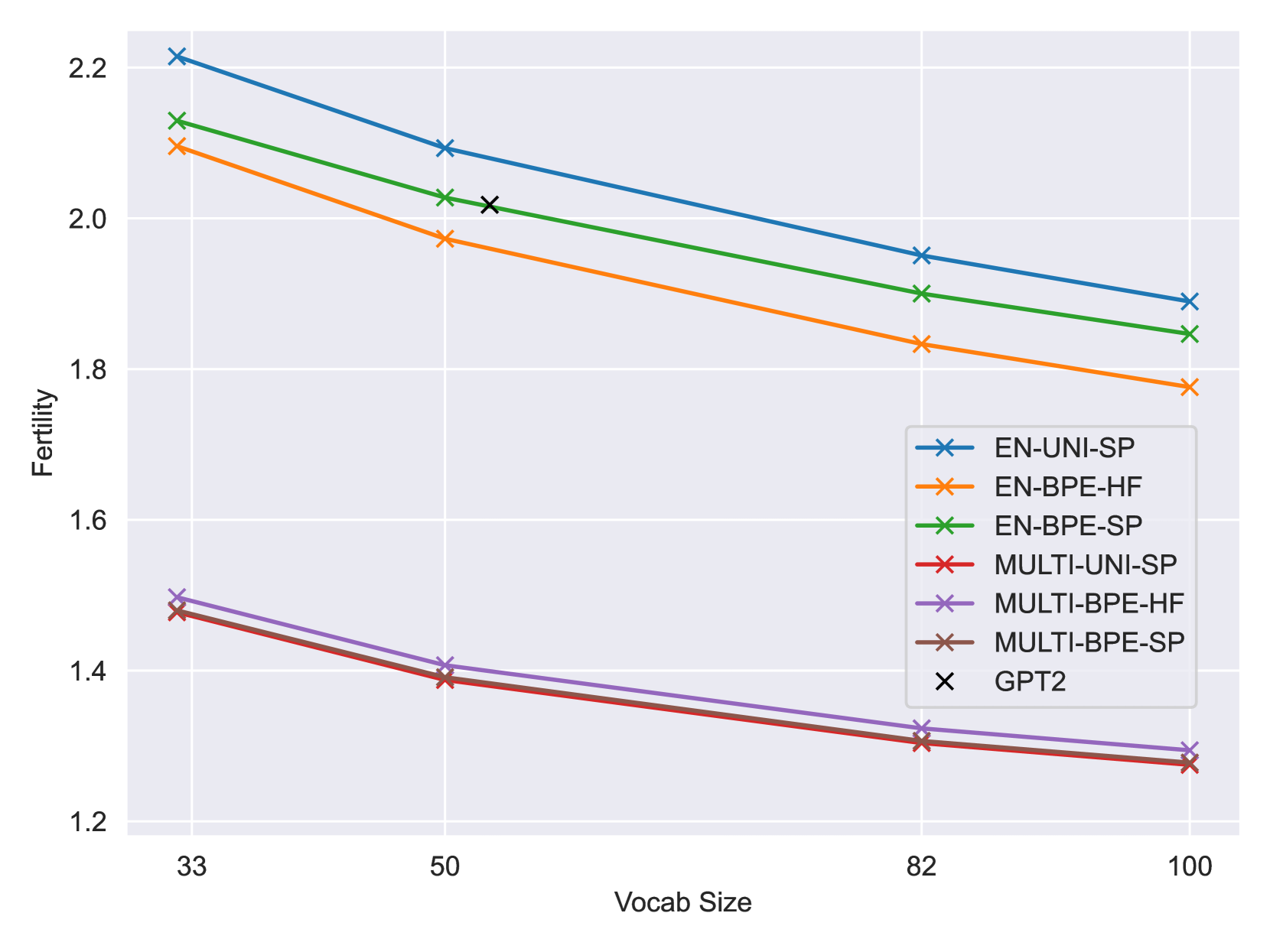
Tokenizer quality
- Choosing the right tokenization is important:
- More tokens -> large embedding matrix
- Longer tokens have less training instances, but better captures semantics
- Longer tokens -> smaller context length
- Tokens must represent well the target texts
- Multilingual LLMs: language specific tokens
- Evaluation with: (lower is better)
- fertility = avg nb of subwords per word
- % of splitted words
BERT tok fertility:
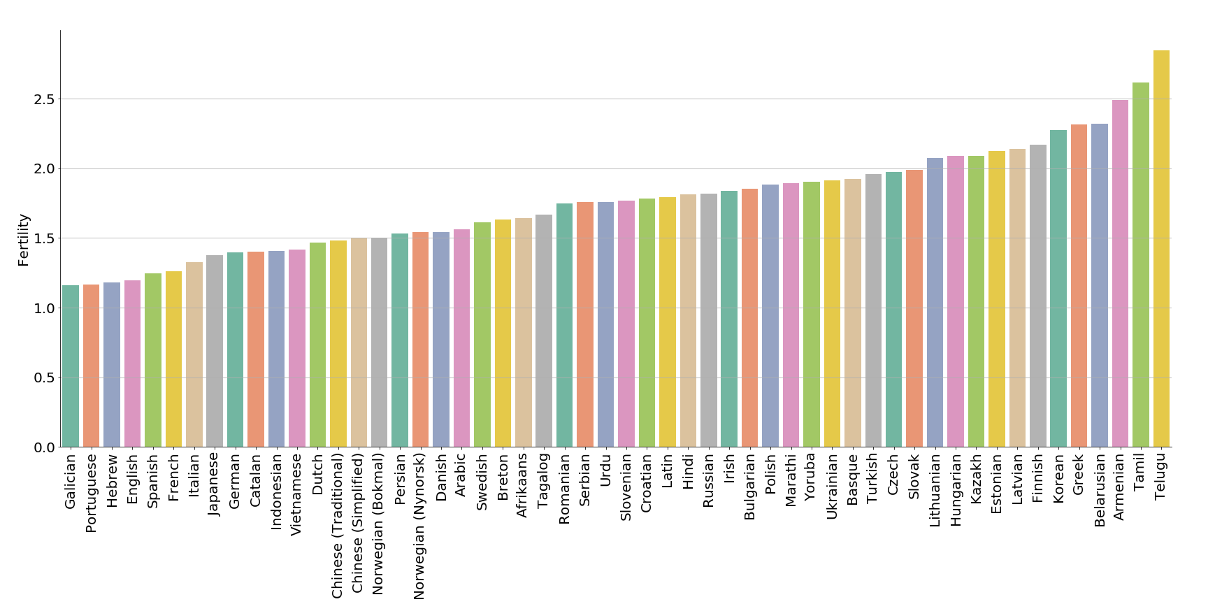
- Fertility smaller (closer to 1) shows that the tokens represent well the language/corpus.
- Comparison of tokenizers:
Tokenizer impact on training costs
- Smaller fertility leads to smaller training costs, but there’s a compromise (Narayanan, 2021):
\[C=96Flh^2\left( 1+\frac s {6h} + \frac V {16lh} \right)\]
\(s=\) sent length, \(l=\) layers, \(h=\) hidden size, \(V=\) vocabulary, \(F=\) fertility, \(C=\) cost per word of 1 forward-backward.
Tokenizer design
- Challenge: repeated long seqs may give 1 token!
- Deduplication during preprocessing
- Best practices: vocab size:
- Bloom: 256k
- GPT3.5: 52k
- Falcon: 64k
- Llama2: 32k
- GPT4: 100k
- Llama3: 128k
- Qwen2: 150k
- Gemma: 256k

Retrieval Augmented Generation
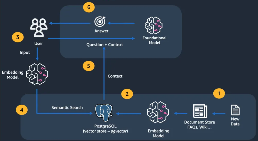
from link
RAG Tools
- llamaindex: specialized for RAG
- langchain
- haystack
- Langroid: LLM agents
- DSPy: prompt optimization
- …
Additional notes
- Warning: terms ambiguity: in a transformer, where are the
“embeddings”?
- Embeddings = fixed, context-independent, per-token, input vectors
- Embeddings = context-dependent, per-sentence vector at the output of the encoder (BERT, CLS token)
- Embeddings (??) = per-sentence vector at the output of the decoder (last token) ?
- Latent representations: per-token activations at the output of some layers
Hands-on
- You may use Jupyter notebooks, but they’re bad from soft. eng. point
of view:
- They’re not designed for GIT
- They’re not designed for collaboration (pair coding, code review, issue tracking, pull requests…)
- They prevent you from adopting soft. eng. best practices: organize codes into files/dirs, decouple core from interfaces, design patterns, unit testing, continuous integration…
So I recommend that you write your code into plain text files and version them in GIT