LLM
- Session 1: intro: impact of LLMs, the 4 revolutions
- Session 2: attention, transformer, KV-cache, anatomy of a prompt
- Session 3: pretraining (scaling laws), PEFT
- Session 4: contrastive training, best practices for training
- Session 5: agentic training
Course requirements:
- Basics of python
- Access to a computer (in & outside class)
- With python + pytorch + transformers installed
- Internet access in & outside class (eduroam)
- Any question:
- christophe.cerisara@loria.fr
- Grading in this course:
- Continuous evaluation
- automatically corrected MCQs
- slides are allowed during MCQs
- But slides do contain very few info! –> take notes of everything else that I say
AI: a bureaucracy revolution
Yuval Harari: Pr. of History at Univ. Jerusalem; Oxford talk
- Some definitions:
- agent: must be able to take decisions, create new things by itself: human, animals, LLM
- agents, like humans, are narrow = adapted to an environment:
- AlphaGo…
- Humans are adapted to the environment created by trees, bacteria…
- AI is adapted to an environment created by humans: language, data, bureaucracy
On the importance of bureaucracy
- humans dominate the world because people cooperate: small 1-to-1 cooperations are frequent, but how to cooperate among 1M people? \(\rightarrow\) bureaucracy like financial, state, churches, universities…
- what do bureaucrats do? they build up trust btw strangers: they have a narrow type of intelligence, but excert an enormous impact on the world: bureaucracy can build cities, erase forests…
AI are native bureaucrats
- AI agents are “native bureaucrats unlike humans”
- in the coming years, AI agents will take over the world’s bureaucracies and make decisions about our lifes
- “is it good or bad?” is not the question: AI agents are much better than us to manage bureaucracy
What are the first jobs taken by modern AIs?
Bureaucracy N°1: social media
- First job taken by AI are news editors
- AIs already have huge influence on the bureaucratic system of social media
- Ais won’t rebel and attack humans, they’ll take over human civilizations from the inside
- When AI’ll control the flow of trust in the world, humans will become spectators and users of an AI financial system they do not understand.
Bureaucracy is language
- Bureaucracy is based on language tokens
- Humans were the only ones to master language
- LLMs are now better than humans at language
- “AIs are hacking the code of human civilization”
- “language is taken away from humans”
“Une étude menée auprès de collaborateurs de l’Assemblée nationale, relayée en avril 2026 par la Fondation Jean-Jaurès, révèle qu’ils sont huit sur dix à utiliser l’IA dans leur travail, dont un sur deux quotidiennement, sans qu’aucune solution officielle ne leur soit fournie.”
LLM: the 4 revolutions of AI
- LLMs are at the core of the AI revolution, because they enable
- exploiting all human knowledge encoded in languages
- reasoning mediated by language
- interacting “naturally” with humans
- 4 main revolutions:
- 2017: the transformer
- 2020: pretraining scaling laws
- 2024: test-time scaling
- 2025: agentic
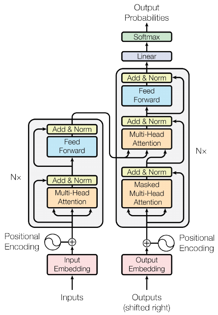
Revolution 1: the transformer (2017)
- Google’s paper: “Attention is all you need”
- Why a revolution? Because it removes important bottlenecks:
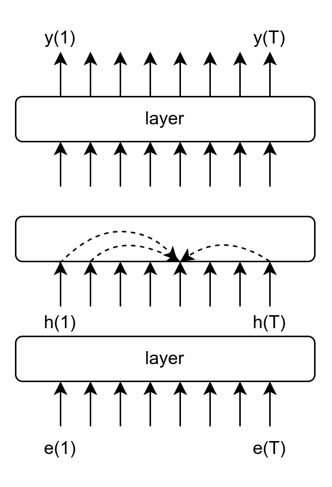
- bottleneck of information in LSTM (h vector encodes all history) and CNN (weighted averaging of embeddings)
- positional bias in LSTM (mitigated by “content-based similarity + positional encodings” for transformers)
- enables parallel computation during training
- Which enables scaling
Sequence of transformations: self-attention (merge concepts) \(\rightarrow\) MLP (memory blocks) \(\rightarrow\) …
Residual stream: each layer adds an \(\varepsilon\) of information
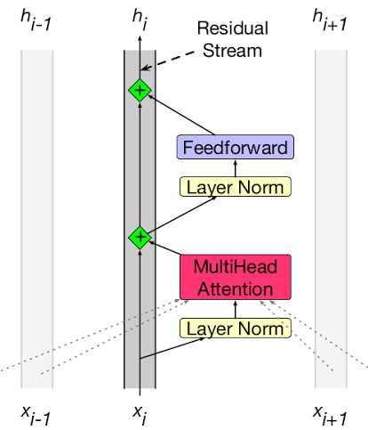
- Modern implementations of transformers improve over the 2017 transformer:
- RoPE, RMSNorm, Pre-Norm, SwiGLU
- GQA, no bias in QKV, long context tricks:
- RoPE scaling, NTK scaling, YaRN, Dynamic scaling, Position interpolation…
- hybrid layers (MoE, Mamba)
- …
Revolution 2: scaling laws (2020)
- First and main LLM scaling laws: pretraining

Scaling LLMs
- The more data you train on
- the more the LLM knows about
- the better the LLM generalizes
- scaling law = power law = \(y(x) = ax^{-\gamma} +b\)
- \(y(x) =\) test loss
- \(\gamma\) = slope
Baidu paper: DNN scaling laws 2017
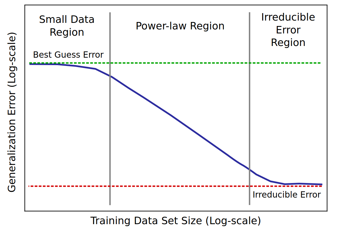
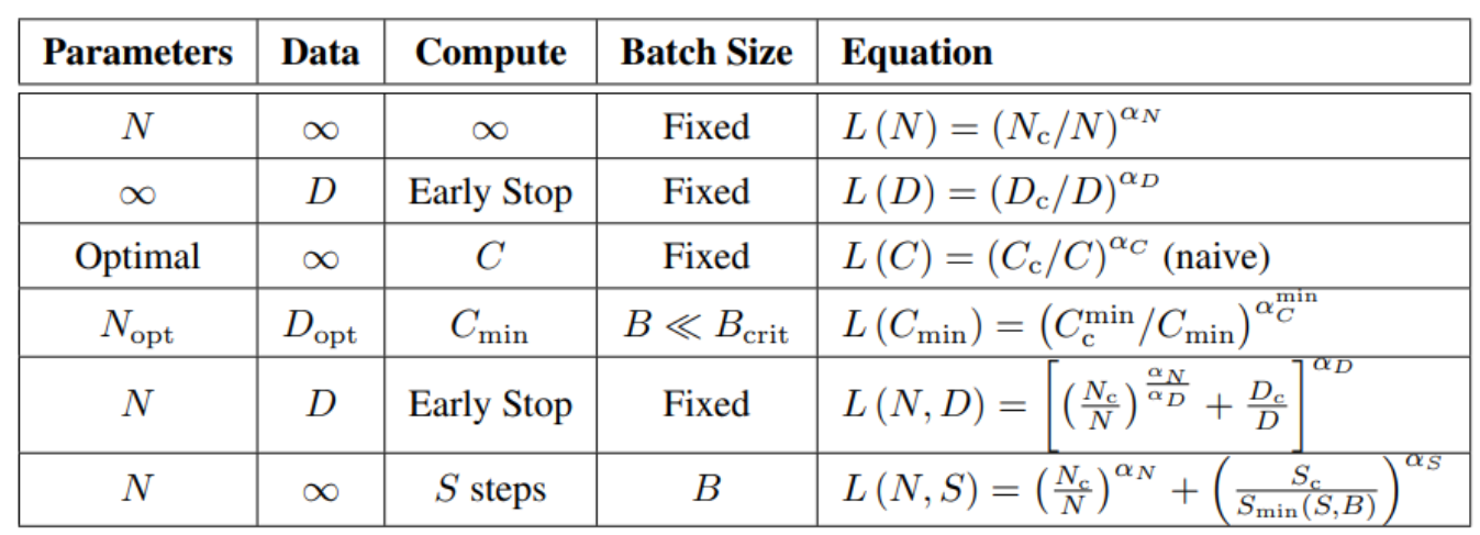
Kaplan scaling laws 2020
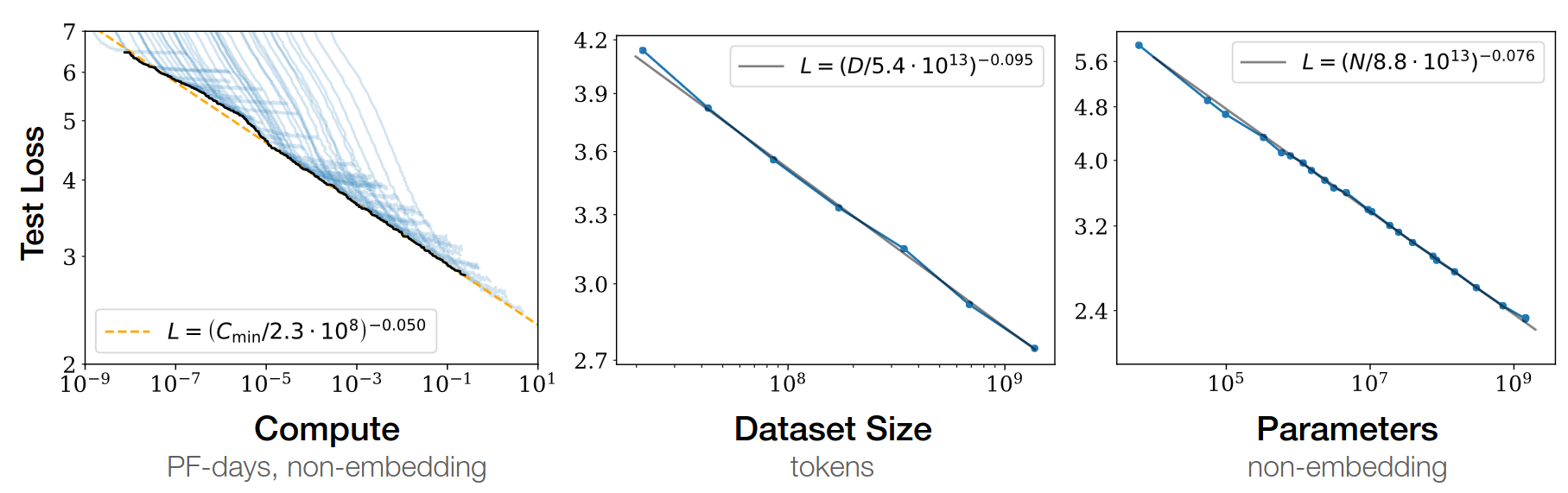
Open-AI 2020
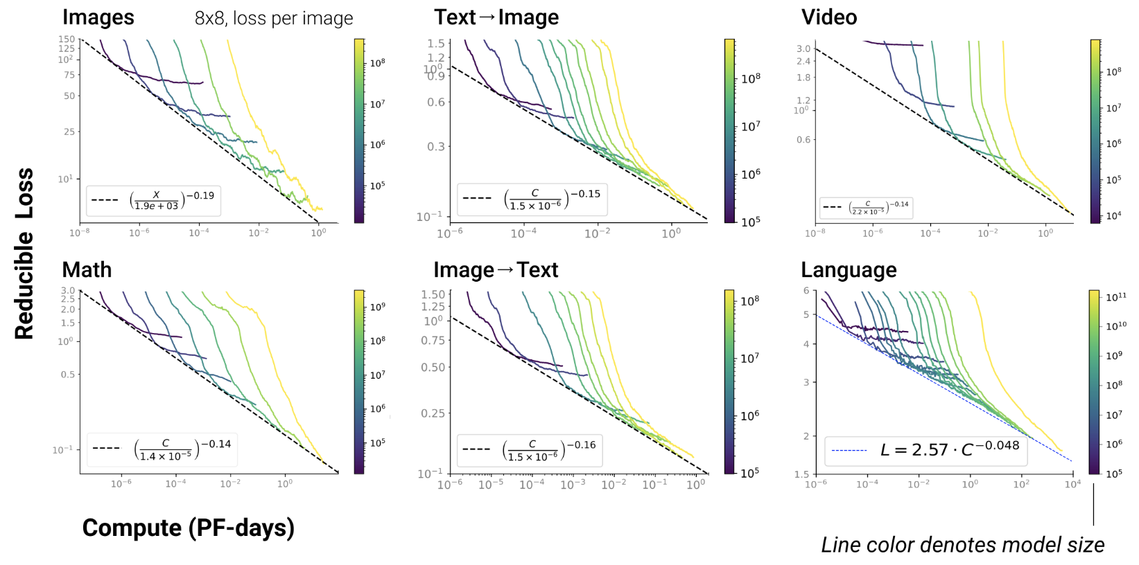
- RL, protein, chemistry…
- Kaplan 2020: you should scale model size
- Chinchilla 2022: you should scale data
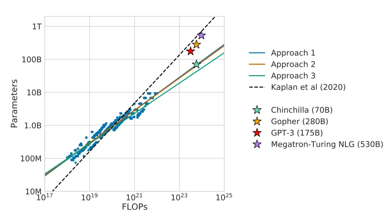
\(L=\) pretraining loss
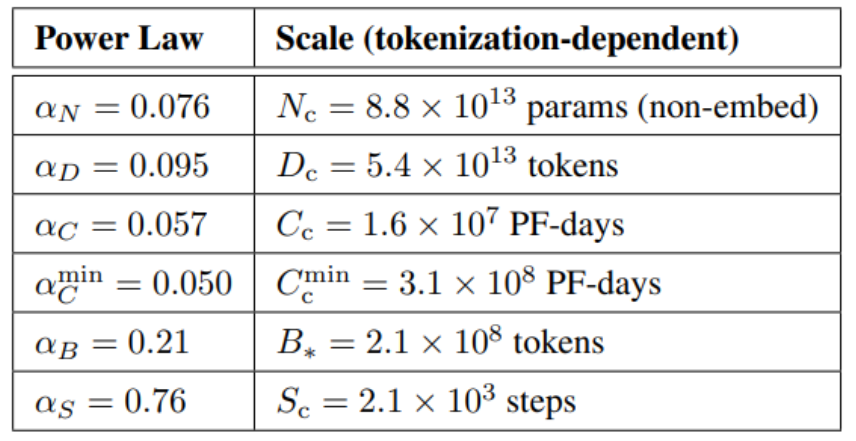
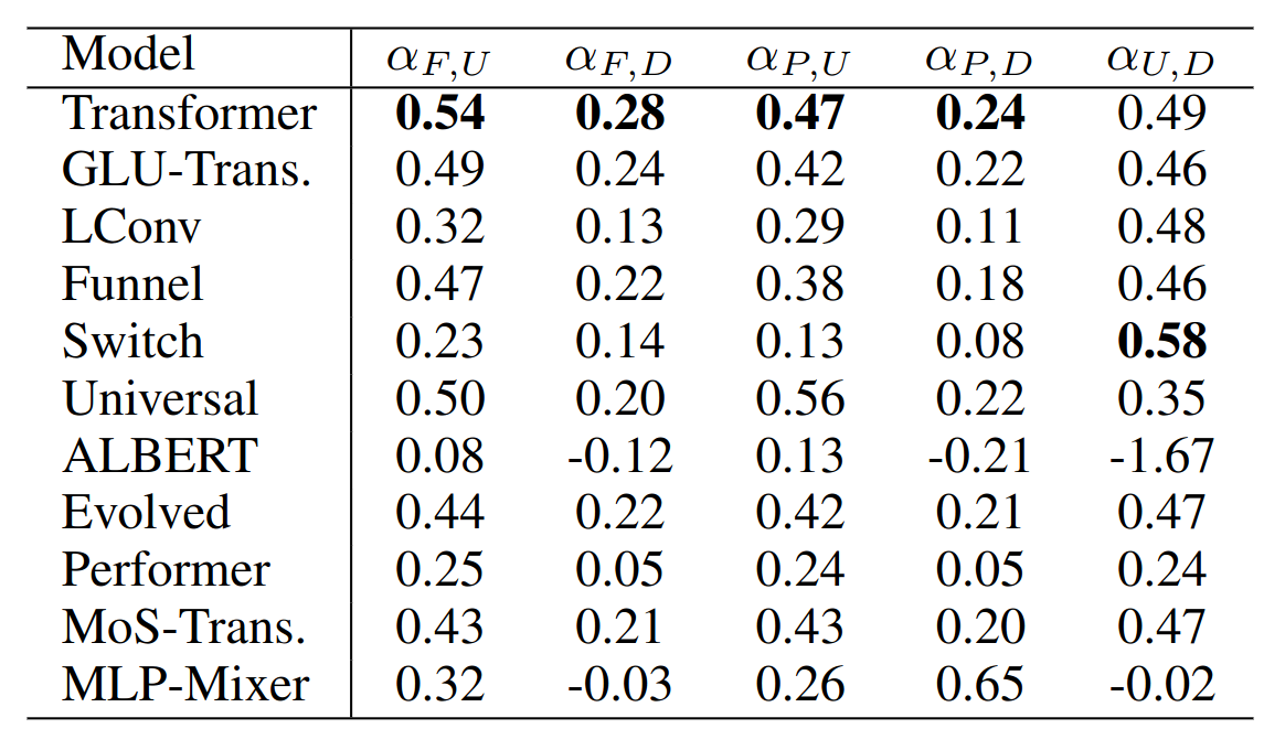
Google: comparison of architectures 2022
Flops, Upstream (pretraining), Downstream (acc on 17 tasks), Params
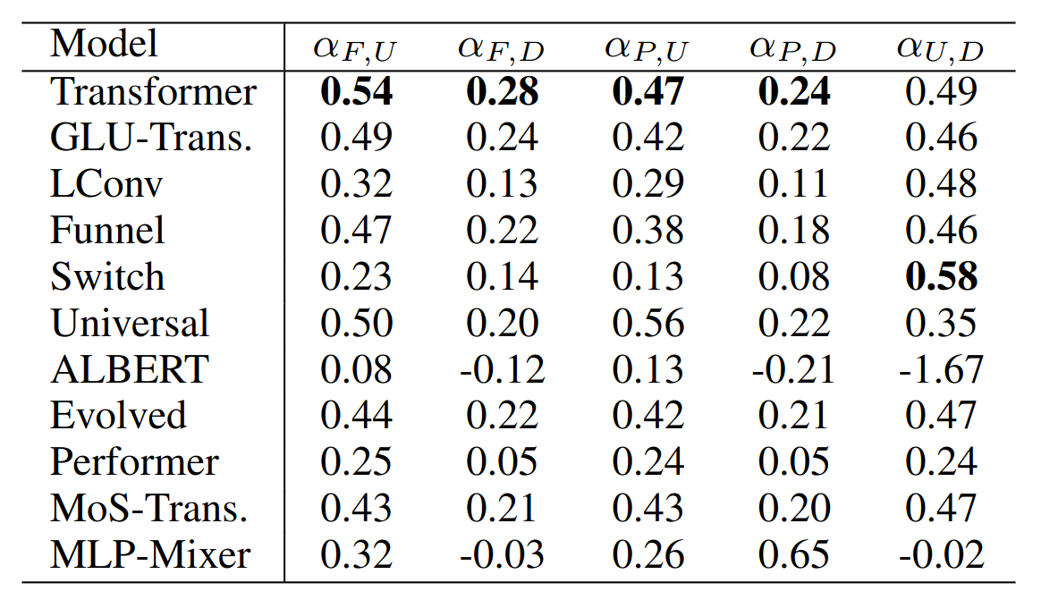
Theoretical limits of linear/hybrid attentions
This paper (2026) proves that linear and hybrid attentions (including Mamba, DeltaNet…) are less expressive than full attention (e.g., for sequential function composition = multi-step reasoning).
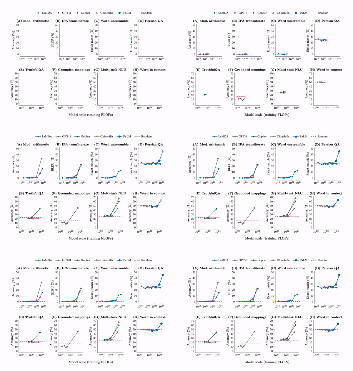
Emerging capabilities
- Scaling laws exist in Machine Learning for a long time (cf. Paper on learning curves)
- But it’s the first time they result from emerging capabilities!
- Most important emerging capability: In-Context Learning 2020
Jason Wei has exhibited 137 emerging capabilities:
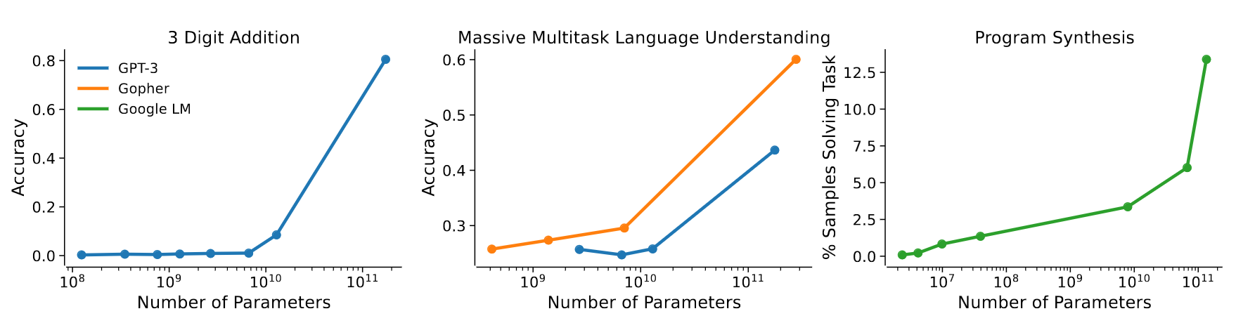
Anthropic paper 2022
- shows that the scaling law results from combination of emerging capabilities
Revolution 3: test-time scaling (2024)
- During training, more compute ==> better results
- During inference: test-time scaling
- Chain of Thoughts (CoT) (2022)
| Method | Core idea | Examples |
|---|---|---|
| Longer reasoning | Longer reasoning | CoT, long reasoning models |
| Sampling | Mult. cand., choose the best | Best-of-N, self-consistency |
| Search | Search in mult. reasoning paths | Tree of Thoughts, MCTS |
| Verification | Generate then verify | Critique-refine |
| Tool use | External computation | Python, search |
| Multi-agent | Collaboration | Debate, solver-verifier |
| Adaptive compute | Spend compute only on hard problems | Dynamic reasoning |
On the “equivalence” between depth and CoT
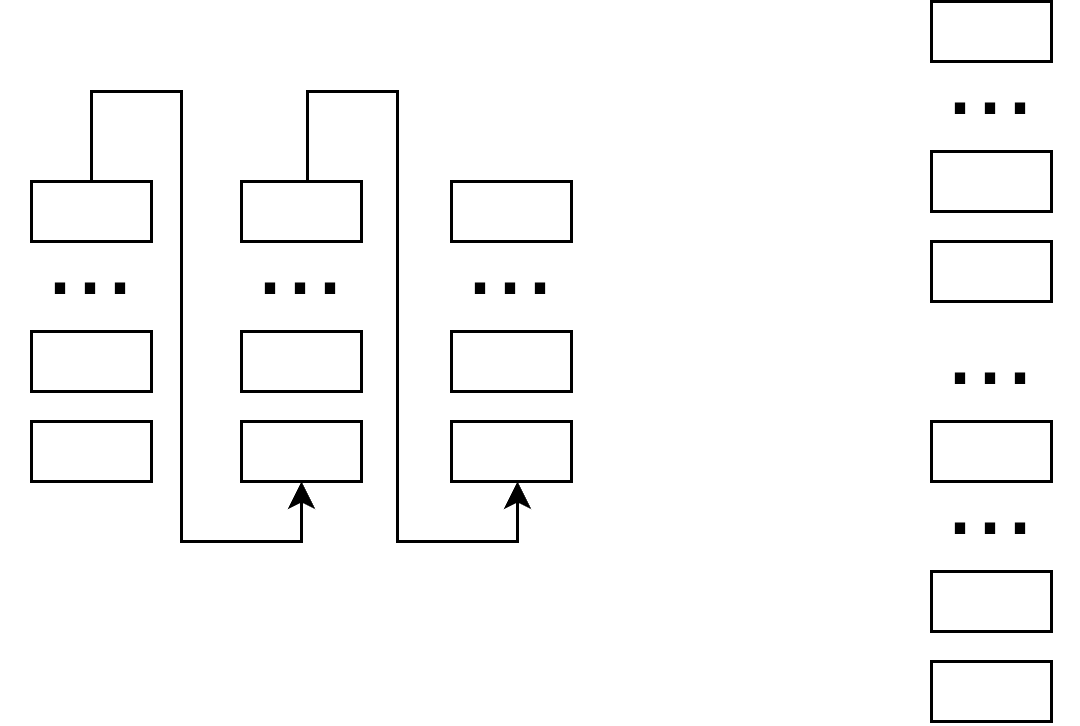
- Can we trade depth for CoT length?
- This depends on the relative expressivity of both:
- Theorem Depth separation: expressivity increases exponentially with depth, poly with width
- Residual expansion theorem: training instability increases exponentially with depth
- Theorem: CoT expressivity:
- CoT(poly(n))=P
- AoT(poly(n))=NP
- CoT(exp(n))=EXP
- AoT(exp(n))=NEXP
- Practical expressivity of CoT:
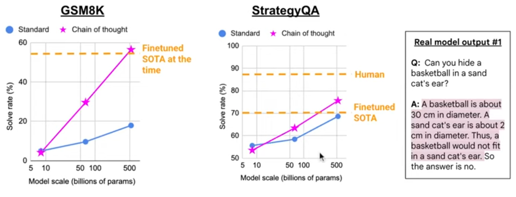
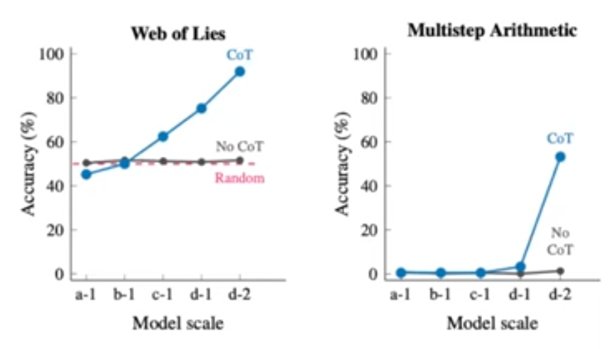
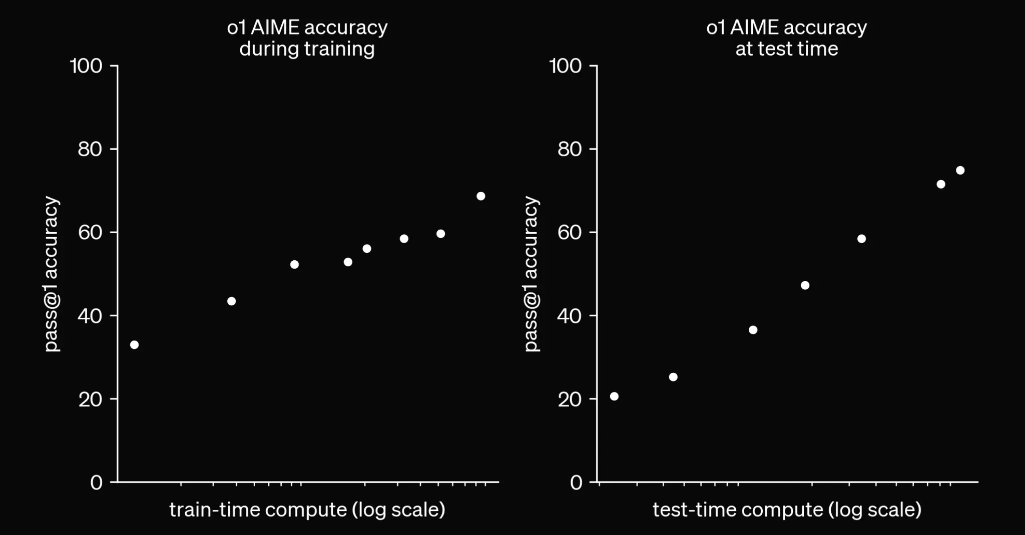
Why does CoT improve results, while it does not bring any new information?
Computer program point of view
- CoT “gives time” (compute) to reason
- “Chain-of-Thought Tokens are Computer Program Variables”
- The transformer is a deterministic (semi-) Turing machine
- With a limited-size ribbon (nb of layers)
- CoT increases ribbon size
- Viewed as program variables, CoT tokens may not be interpretable!
- CoT is not required to be correct: Beyond Semantics: The Unreasonable Effectiveness of Reasonless Intermediate Tokens
- But it does help when it is correct: Probing the Trajectories of Reasoning Traces in LLM
How do LLMs learn to reason?
Are LLMs stochastic parrots?

Or do they really reason?
- There is no reasoning without generalization
- Compression = generalization
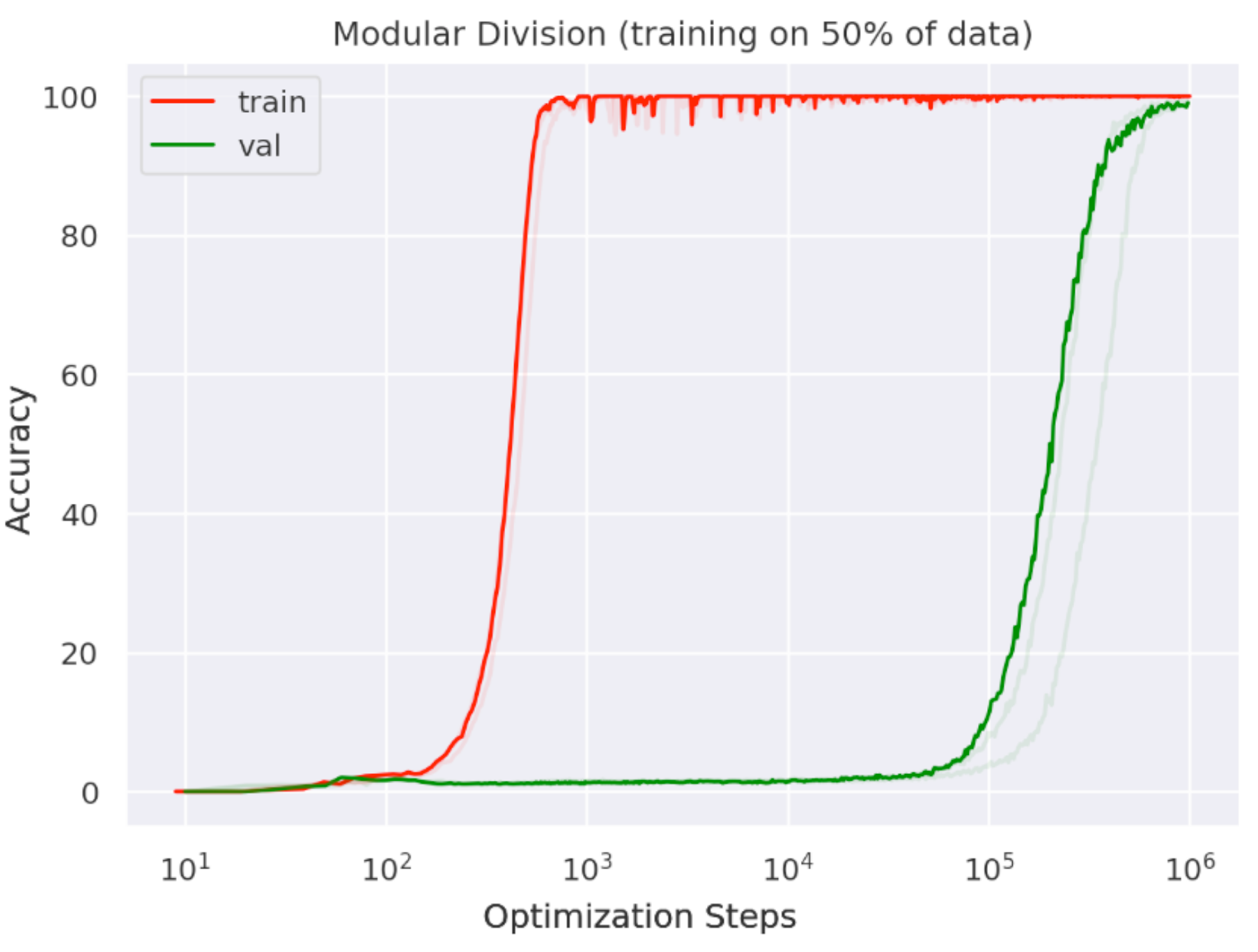
- During DNN/LLM training, 2 phases occur: memorisation, then generalization
- Tishby, 2015
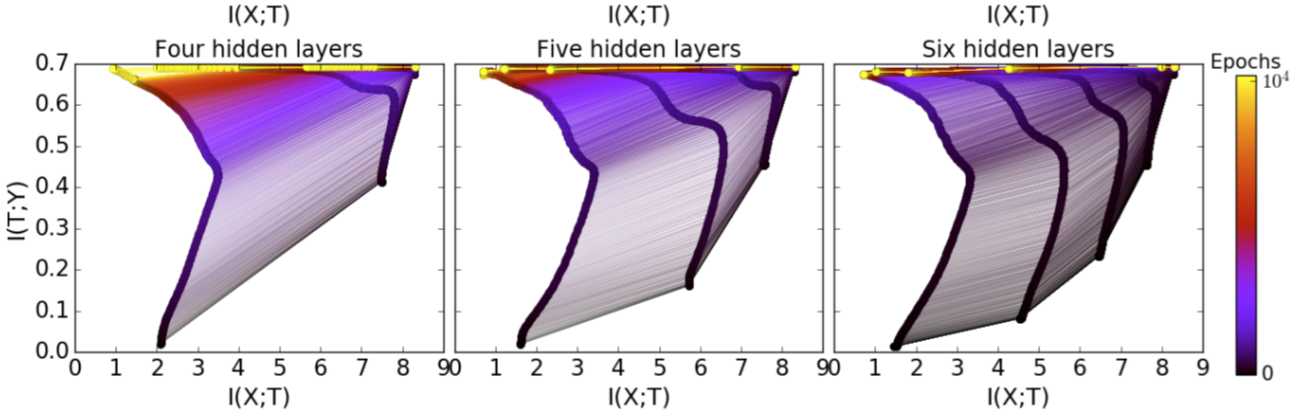
Phase transitions during training
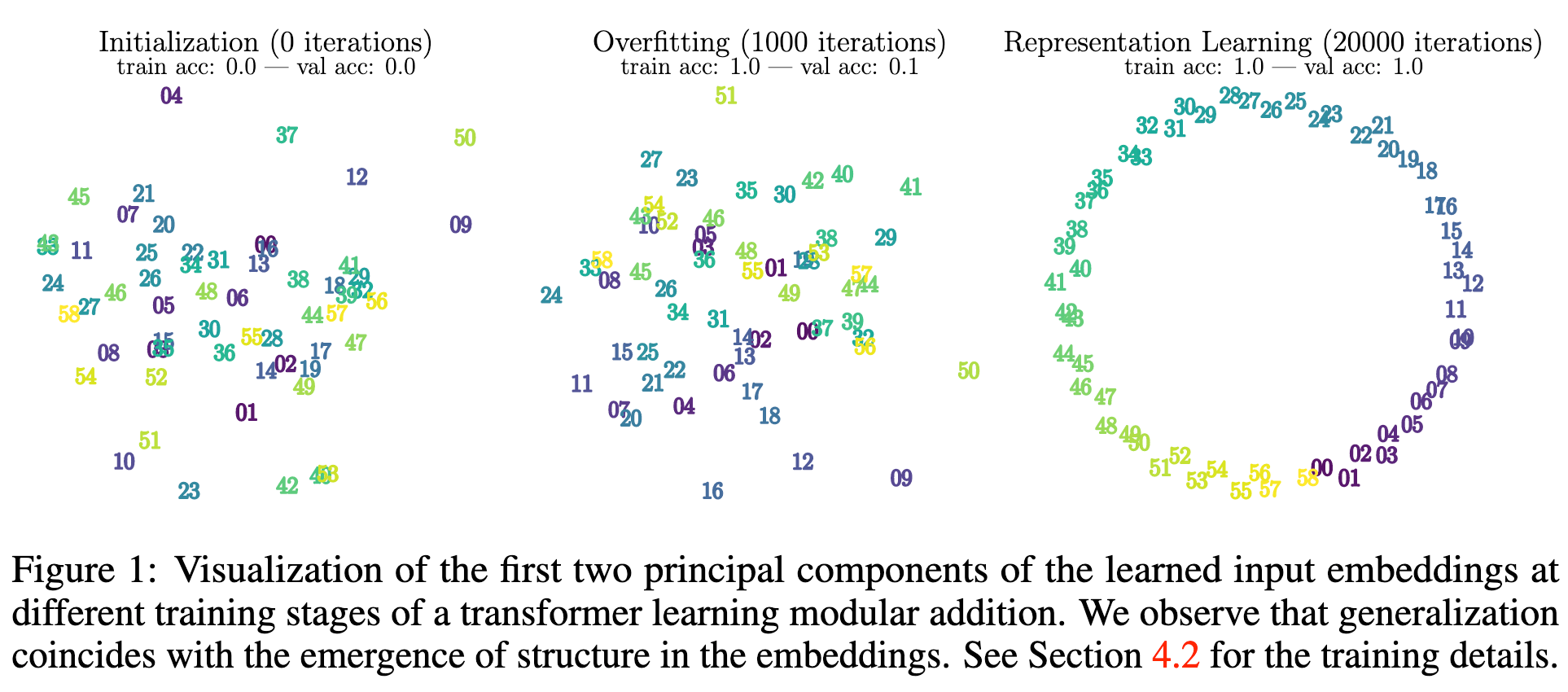
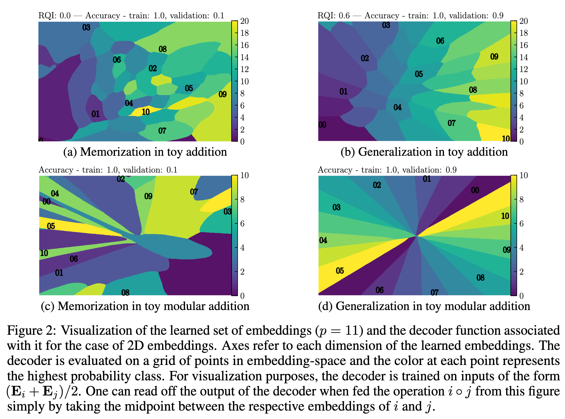
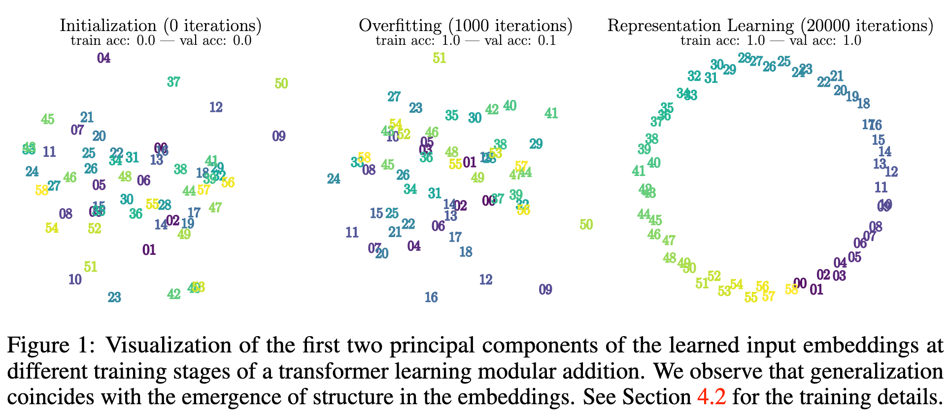
Grokking exhibits structured latent space; Ex: modular arithmetic
LLM training dynamics
- High-dim training is not a “continuous”/regular process:
- Phase transitions first observed in 2015 in ConvNets
- Later studied in LLMs
- LLMs generalize by discovering the latent structure in data
- World geography emerge
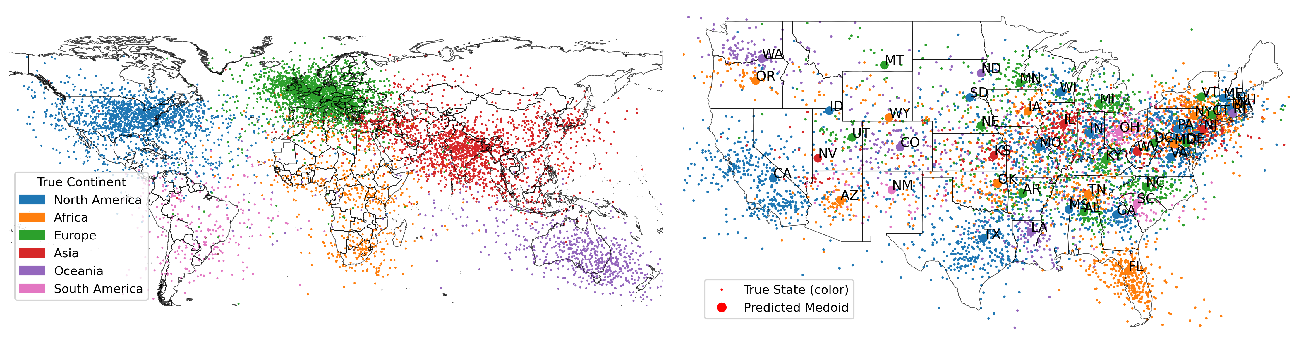
- LLMs learn to learn (in context):
- So, we know that LLM can:
- not only memorize, but generalize
- recover latent structures in data
- learn training algorithms
- execute these algorithms in their residual stream
- Do they actually do that when generating CoT?
“Procedural Knowledge in Pretraining Drives Reasoning in Large Language Models”
“The approach to reasoning LLMs use looks unlike retrieval, and more like a generalisable strategy synthesising procedural knowledge from many documents doing a similar form of reasoning.”
- Method: Influence functions identify which training data is used when reasoning
- Influence functions: assume removing a training doc, retrain, does prediction change?
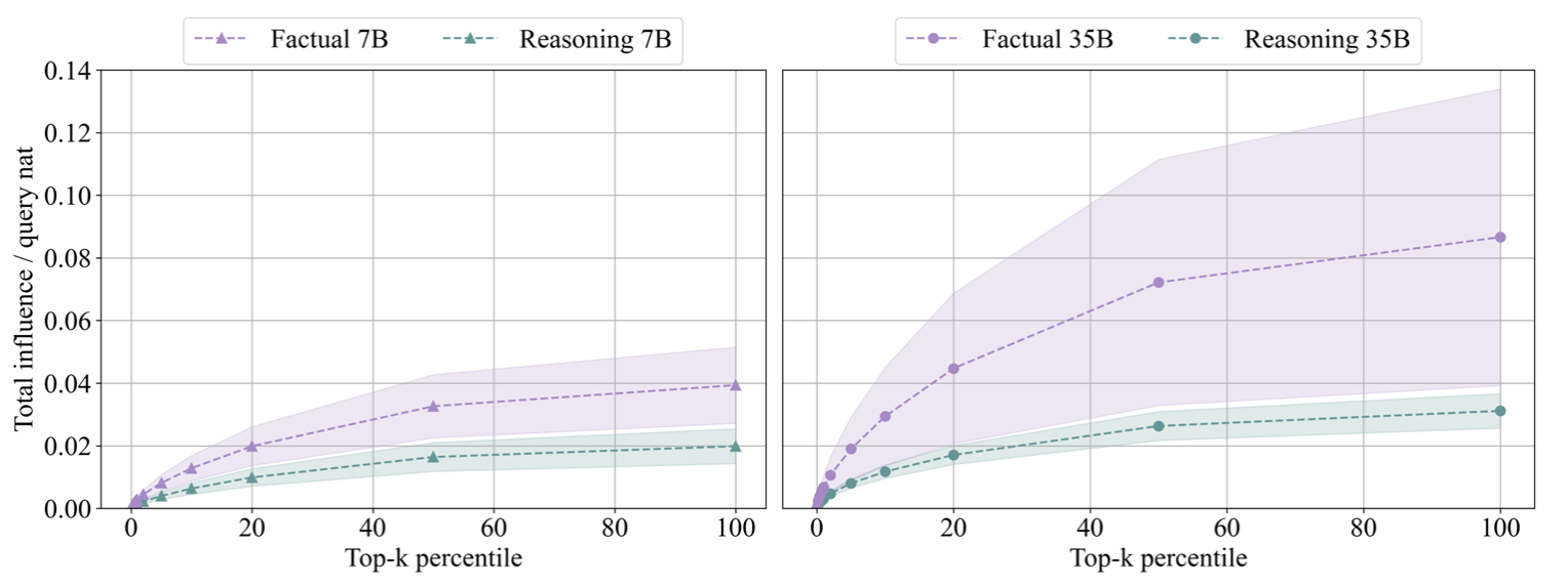
Reasoning Qs are weakly influenced by individual docs; factual Qs are.
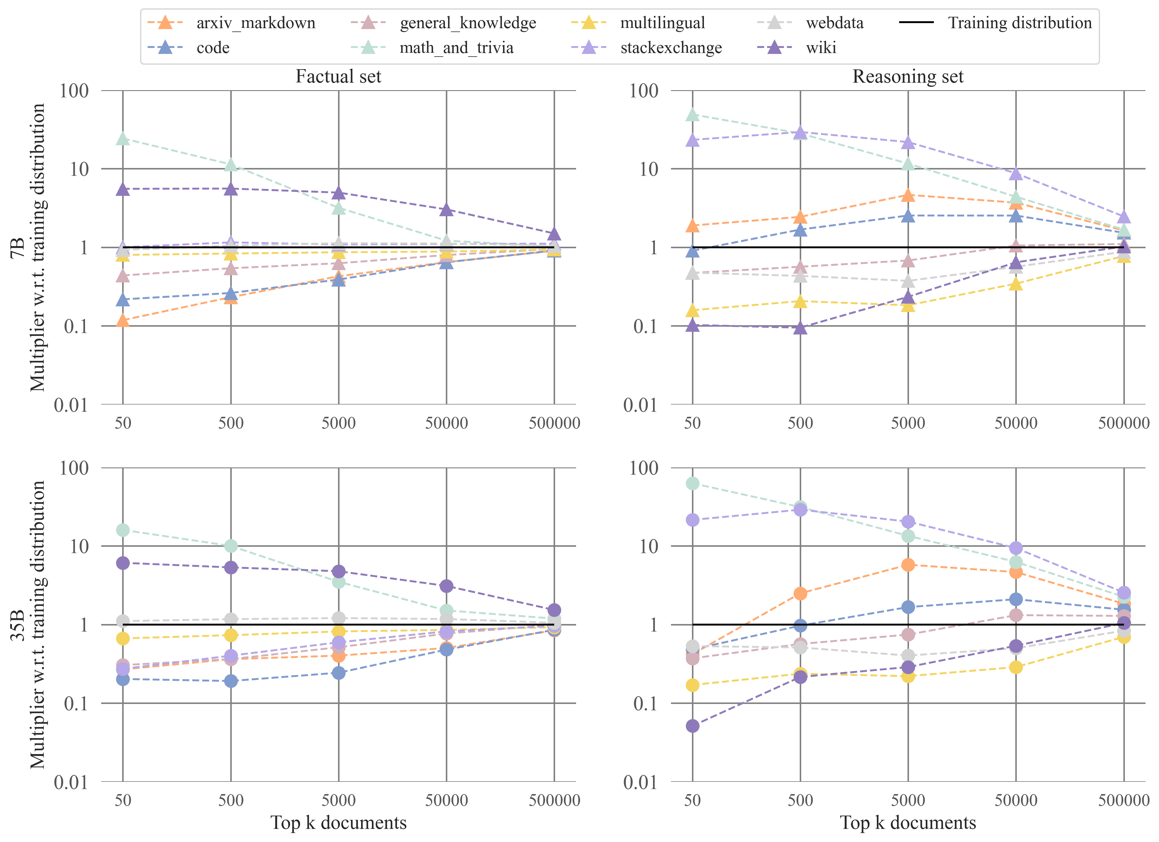
- Reasoning Qs are mostly influenced by code datasets
- Factual Qs are mostly influenced by wikis
- Additional refs:
- Transformers Pretrained on Procedural Data Contain Modular Structures for Algorithmic Reasoning
- Scalable Influence and Fact Tracing for Large Language Model Pretraining
When are LLMs trained to reason?
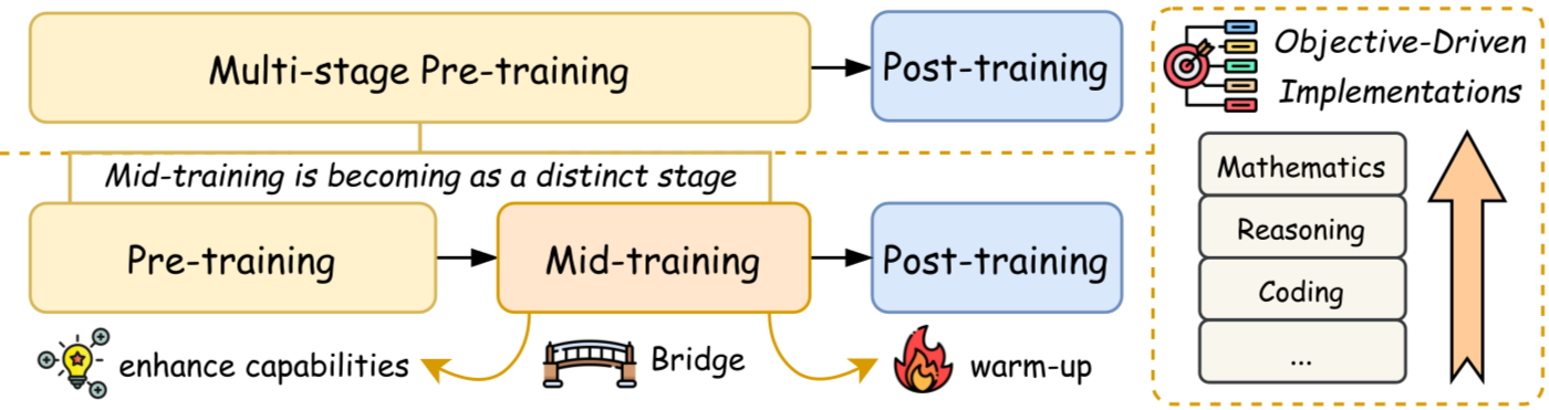
- Pre: No explicit CoT
- Mid: Supervised CoT (often distilled)
- Post: Generated CoT (RL)
- RL with CoT improve performance on reasoning benchmarks e.g. “Effective Reinforcement Learning for Reasoning in Language Models”
- Q1: Does RL inject novel reasoning capacities into LLM?
- Q2: Can we reduce the large cost of RL?
- RL may be replaced by high Quality supervised CoT:
- S1 (feb 2025): good performances with 1000 manual CoT
- Distillation: always train an LLM (without RL) on high quality CoT generated by top-LLMs
Reasoning capacities are already in the base LLM (before post-training)
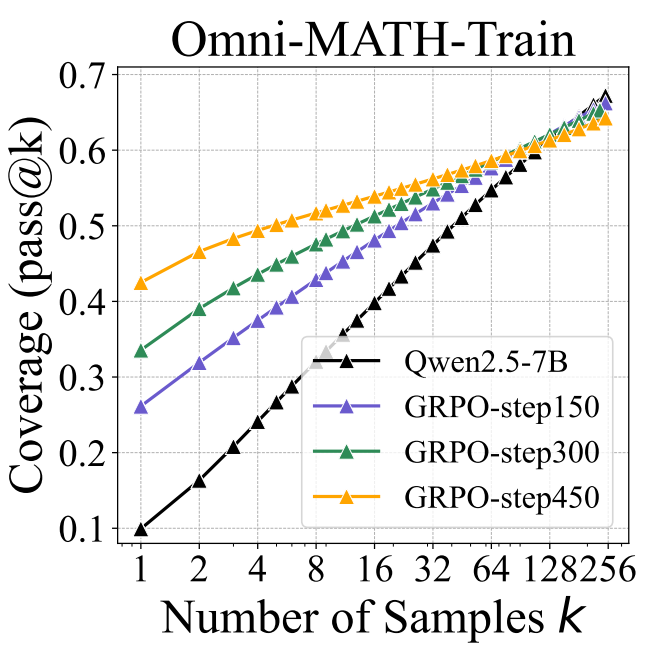
- Before RL, correct answer is not always first, but is not far
- They checked manually that base LLM generates CoT that are as valid as post RL
- Tested on maths, code, visual reasoning
- Base LLM can potentially solve more problems than after RL

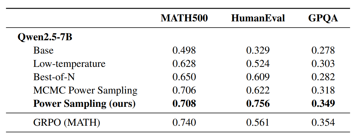
- RL does not add any new reasoning capacity, but “sharpen” the distribution \(p(x)^{\alpha}\)
- Without RL, one can draw CoT with MCMC from \(p(x)^{\alpha}\) instead of \(p(x_t | x_{<t})\)
- But MCMC is costly (x9), this paper proposes an efficient approximation
- Other lessons of the paper:
- RL induces a “diversity collapse”
- \(\alpha\) impacts performance: \(\alpha=4\) is a good value for maths
- CoTs are in English, because all reasoning datasets are in English, as well as generated CoTs. \(\rightarrow\) Mille-Pensées

Revolution 4: agentic (2025)
AI Agent: LLM + harness + agentic loop
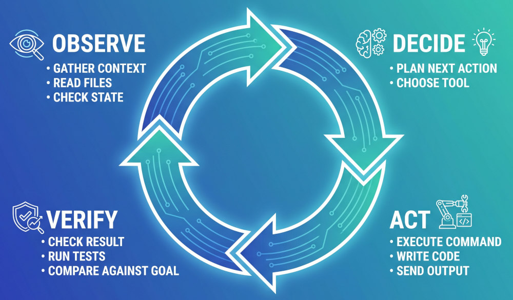
harness: all the code around the LLMs
- Why a revolution?
- Because, thanks to trial and errors, debugging, planning, agentic AI enables to solve much more complex tasks than a single LLM
- The LLM is trained to run tools and analyze their outputs, try to understand why it failed, debug the process, rerun until it works
- Ex: solved one of the 10 major Erdös problem
Training an agentic LLM requires moving beyond standard text corpora. While a base LLM needs general language understanding, an agent specifically requires data that teaches reasoning, planning, tool usage, environment interaction, and multi-turn error recovery.
Standard training pipeline to train an agent: Pre-training → Agentic SFT → RLVR
Agents orchestration
- Various types of orchestration
- Central: main LLM = orchestrator
- Hierarchic: several levels of orchestrators
- “Control graph”: controlled programmatically
- Swarm: many small specialized LMs
Opportunity for small LLMs
- More and more “small” focused LLMs are developed
- for code: 3b LLM
- for repository exploration: Microsoft 4b LLM
- for agentic loop: Ornith 9b
- for long-horizon planning: Agents A1 35b
Attention
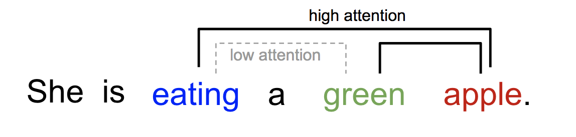
- Intuition: transform word emb. using related context words
- See Lilian Weng blog
| Year | Authors | Contribution |
|---|---|---|
| 2014 | Graves et al | attention for Neural Turing Machines |
| 2014 | Bahdanau attention | application to NLP |
| 2015 | Luong attention | application to NLP |
| 2015 | Xu et al. | soft/global & hard/local |
| 2016 | Cheng, Dong and Lapata | self-att LSTMN |
| 2017 | Vaswani et al. | transformer, 120k citations |
Common general form: QKV
\[\begin{equation} {\scriptsize{ \alpha_i = \frac {\exp(\text{score}(q,k_i))} {\sum_j \exp(\text{score}(q,k_j))} }} \end{equation}\] \[\begin{equation} {\scriptsize{ v' = \sum_i \alpha_i v_i }} \end{equation}\]
Similarity score
| name | score | ref |
|---|---|---|
| content-based | cosine\((q,k)\) | Graves14 |
| additive | \(v^T \tanh (W[q,k])\) | Bahdanau15 |
| location-based | \(\alpha = \text{softmax}(Wq)\) | Luong15 |
| general | \(q^T W k\) | Luong15 |
| dot-product | \(q^T k\) | Luong15 |
| scaled \(\cdot\) | \(\frac {q^t k} {\sqrt{d}}\) | Vaswani17 |
Scaled dot-product?
- Assume input E[k]=0 var(k)=1 \[var(xy) = (var(x)+E[x]^2)(var(y)+E[y]^2) - E[x]^2E[y]^2\]
- \(k\) and \(q\) independent: \(E[kq]=E[k]E[q]=0\) \[var(k_i q_i) = (var(k_i)+E[k_i]^2)(var(q_i)+E[q_i]^2) - E[k_i]^2E[q_i]^2 = 1\]
- Output variance: \[var\left(\sum_i k_iq_i\right) = \sum_i var(k_iq_i) = d\]
Self-attention
- Cheng 2016: use same sentence both for K and Q
- Often represented by a heat map over the words of the sentence
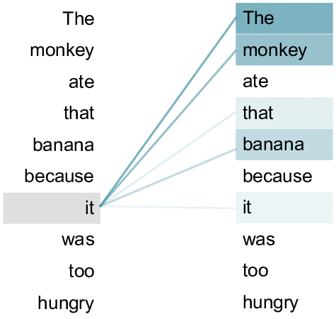
- Is attention interpretable? Does it enable explainability?
- No: cf. Why Attentions May Not Be Interpretable?
- Combinatorial shortcuts: attention carry extra info for next layers
- Other approaches: Integrated gradients, SHAP, Layer-Wiser Relevance Propagation, Causal tracing…
Matrix formulation
- arrange all keys \(k_i\) as a matrix \(K \in R^{N \times d}\)
- each vector \(k_i\) is a row of the matrix
- same for all queries \(q_i\) as \(Q \in R^{N \times d}\)
- \(A=\)softmax\((QK^T)\)
- for each row, column, or globally?
- This matrix product outputs the new V = weighted sum of original V
- Beware of dimensions!
Self-attention with scaled dot-product:
\[V'=\text{softmax}\left(\frac {QK^T}{\sqrt{d}}\right)V\]
Cost
- The cost of \(QK^T\) is in \(O(n^2d)=O(n^2)\) operations
- But each of the \(n^2\) dot products can be computed in parallel, so we have \(O(1)\) sequential operations
- Transformers are well adapted to GPU!
- Compare to RNN: \(O(n)\) sequential operations
from https://slds-lmu.github.io/seminar_nlp_ss20/attention-and-self-attention-for-nlp.html
| Layer | Complexity | Seq. op |
|---|---|---|
| recurrent | \(O(nd^2)\) | \(O(n)\) |
| conv | \(O(knd^2)\) | \(O(1)\) |
| transformer | \(O(n^2d)\) | \(O(1)\) |
| sparse transf | \(O(n\sqrt{n})\) | \(O(1)\) |
| reformer | \(O(n\log n)\) | \(O(\log (n))\) |
| linformer | \(O(n)\) | \(O(1)\) |
| linear transf. | \(O(n)\) | \(O(1)\) |
Attention mask
- When the decoder is trained on sentence “The cat sat on the mat”, every seq is used to learn the next word:
- the –> cat
- the cat –> sat
- the cat sat –> on
- …
- This is causal LM
- We could give the decoder 6 sub-sentences (“The”, “The cat”, …)
- But it’s more efficient to give it the full sentence, and train with a causal mask:
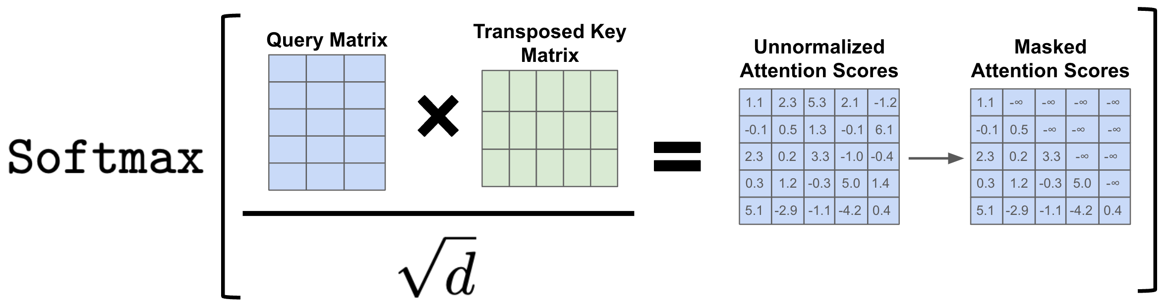
Inference: KV cache
\[Q,K \in R^{N\times d}\] \[QK^T \in R^{N\times N}\]
- So storing \(QK^T\) requires \(O(n^2)\) memory
- A decoder (GPT) generates each token with auto-regression:
- Each step recomputes self-att on the same sentence plus one word!
- Solution: save the already computed \(K\) and \(V\):
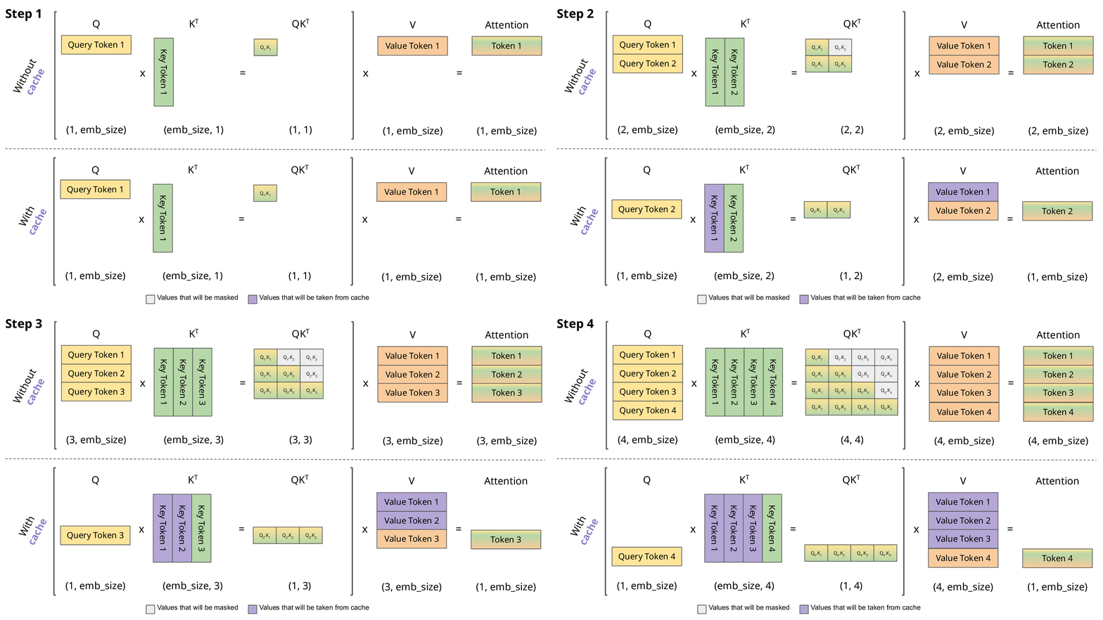
KV cache
- KV cache leads to
- faster matrix computations
- more memory to store cache
- New enhancements:
- KV cache quantization
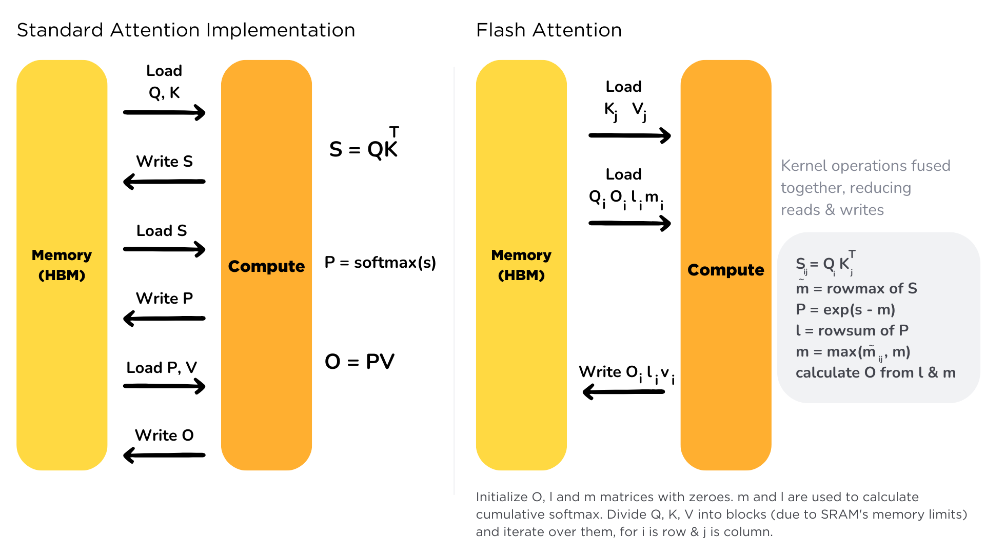
Flash Attention
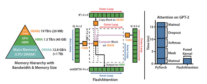
- Bottleneck: memory I/O
- High Bandwidth Memory = large but slow
- GPU on-chip SRAM = small but fast
- kernel = function that runs on GPU
- fused kernels: ex: selfatt scale, mask, softmax
- Other frameworks: xFormers, FasterTransformer, TensorRT-LLM, PyTorch 2.x
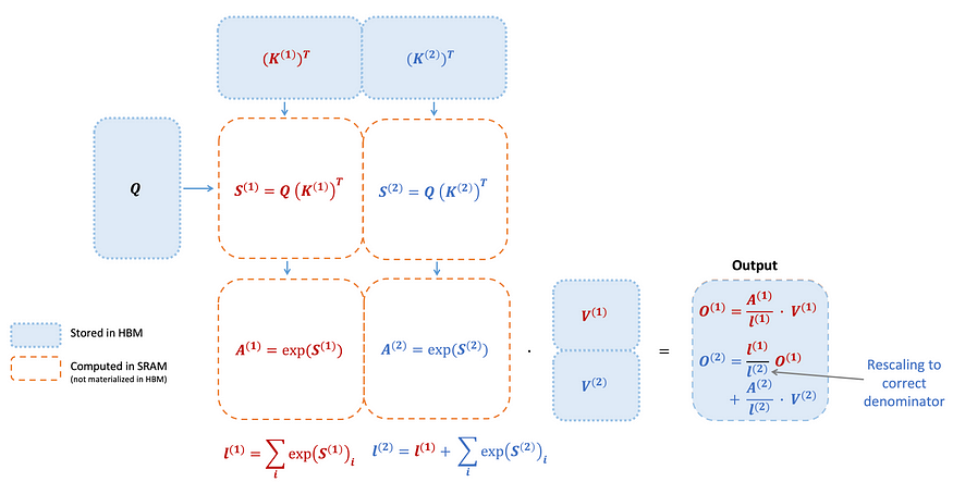
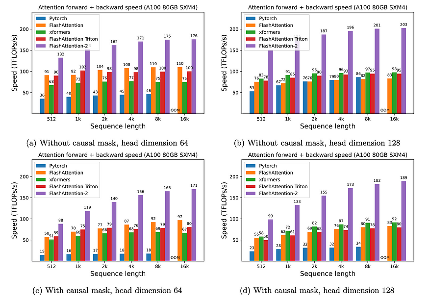
Flash Attention 2
- Divides and parallelizes the computation with the K and V matrices
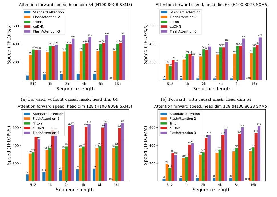
Flash Attention 3
- adapted to H100 GPU
- overlap warped matmuls and softmax
- FP8 “incoherent processing” (see QuiP) = multiplies the query and key with a random orthogonal matrix to “spread out” the outliers and reduce quantization error
- Sliding Attention
- Grouped-Query Attention (GQA): 8x memory reduction at inference video
- Radix Attention
- Paged Attention
- Flex-Attention
- Grouped Differential Attention
- Kimi Delta Attention
- …
Kernel optim on CPU
matmul on python: 0.042 GFLops
numpy (FORTRAN): 29 GFlops
reimplementation of numpy in C++: 47 GFlops
BLAS with multithreading: 85 GFlops
llama.cpp (focus matrix-vec): 233 GFlops
Intel’s MKL (closed source): 384 GFlops
OpenMP(512x512 matrix): 810 GFlops
exported in llamafile: 790 GFlops
Matmult optimisation on CPU
From James Ma website
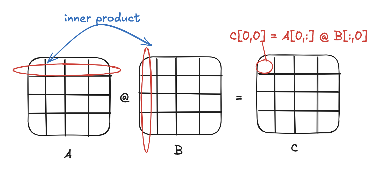
float *matmul_naive(float *A, float *B) {
    float *C = new float[rowsA * colsB];
    float tmp;
    for (int rowA = 0; rowA < rowsA; ++rowA) {
        for (int colB = 0; colB < colsB; ++colB) {
            tmp = 0.0;
            for (int colA = 0; colA < colsA; ++colA) {
                tmp += A[rowA * colsA + colA] * B[colA * colsB + colB];
            }
            C[rowA * colsA + colB] = tmp;
        }
    }
    return C;
}
dim=1024, 3.71s
Linear combination of rows: the CPU reads and caches a whole row of B, so we should use the whole row B before switching to the next one:
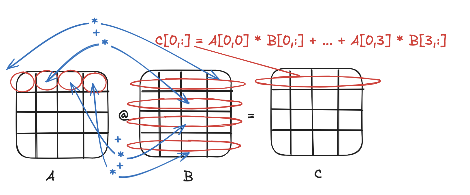
float *matmul_loop_reordered(float *A, float *B) {
    float *C = new float[rowsA * colsB];
    for (int rowA = 0; rowA < rowsA; ++rowA) {
        for (int colA = 0; colA < colsA; ++colA) {
            for (int colB = 0; colB < colsB; ++colB) {
                C[rowA * colsA + colB] +=
                    A[rowA * colsA + colA] * B[colA * colsB + colB];
            }
        }
    }
    return C;
}
3.71s down to 1.62s
But we read the first row B again and again at each outer iteration: Let’s do the next iteration asap! sum of outer products:
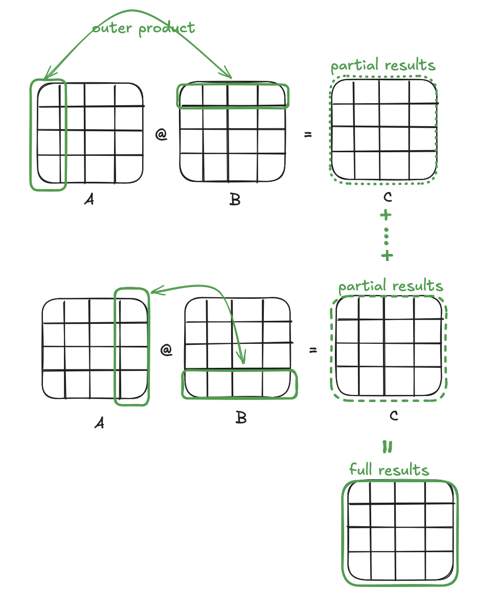
float *matmul_tiled(float *A, float *B) {
    float *C = new float[rowsA * colsB];
    // multiply A[:, tile * tile_size : (tile + 1) * tile_size]
    // and B[ tile * tile_size : (tile + 1) * tile_size ,:]
    for (int tile = 0; tile < colsA / tile_size; ++tile) {
        for (int rowA = 0; rowA < rowsA; ++rowA) {
            for (int colA = tile*tile_size; colA<(tile+1) * tile_size; ++colA) {
                for (int colB = 0; colB < colsB; ++colB) {
                    C[rowA * colsA + colB] +=
                        A[rowA * colsA + colA] * B[colA * colsB + colB];
                }
            }
        }
    }
    return C;
}
1.62s down to 1.60s
Multithreading:
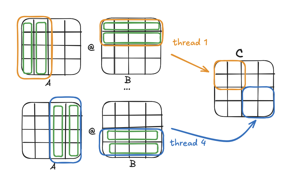
void kernel(float *A, float *B, float *C,
        int start_row, int end_row, int start_col, int end_col) {
    for (int tile = 0; tile < colsA / tile_size; ++tile) {
        for (int rowA = start_row; rowA < end_row; ++rowA) {
            for (int colA=tile*tile_size; colA<(tile+1)*tile_size; ++colA) {
                for (int colB = start_col; colB < end_col; ++colB) {
                    C[rowA * colsA + colB] +=
                        A[rowA * colsA + colA] * B[colA * colsB + colB];
                }
            }
        }
    }
}

float *matmul_multithreaded(float *A, float *B) {
    float *C = new float[rowsA * colsB];
    int start, end;
    int block_size = rowsA / sqrt(num_threads);

    std::vector<std::thread> threads;
    int start_row, end_row, start_col, end_col;
    for (int row = 0; row < sqrt(num_threads); ++row) {
        start_row = row * block_size;
        end_row = row * block_size + block_size;
        for (int col = 0; col < sqrt(num_threads); ++col) {
            start_col = col * block_size;
            end_col = col * block_size + block_size;
            threads.push_back(
                std::thread(kernel<rowsA, colsA, colsB, tile_size>, A, B, C,
                    start_row, end_row, start_col, end_col)
            );
        }
    }
    for (auto &thread: threads) {
        thread.join();
    }
    return C;
}
4 threads: 1.6s down to 0.46s
Hands on
Transformer
- Transformer: (Vaswany et al., Google, 2017)
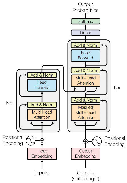
Details of the stack
- Bottom:
- convert input tokens to static embedding vectors \(X_t\)
- table lookup in Embeddings matrix
- Embeddings trained along with all other parameters (\(\neq\) contrastive)
- 3 matrices transform input embeddings \(X\) into \(Q,K,V\)
- convert input tokens to static embedding vectors \(X_t\)
Positional Encodings
- Self-attention gives the same repr when you shuffle the words !
- Inject information about position through a vector that encodes the position of each word
- Fixed absolute position is a bad idea
- Trainable absolute position is OK
- Better: relative fixed positions
- Early relative positional encodings
- Alibi
- ROPE
- …
- Early relative positional encodings
- inspired by spectral analysis
- positions are encoded along sinusoidal cycles of various frequencies
\[p_t^{(i)} = \begin{cases} sin(w_k \cdot t), \text{if }i=2k \\ cos(w_k \cdot t), \text{if }i=2k+1 \end{cases}\]
with \(d\) encoding dim and
\[w_k = \frac 1 {10000^{2k/d}}\]
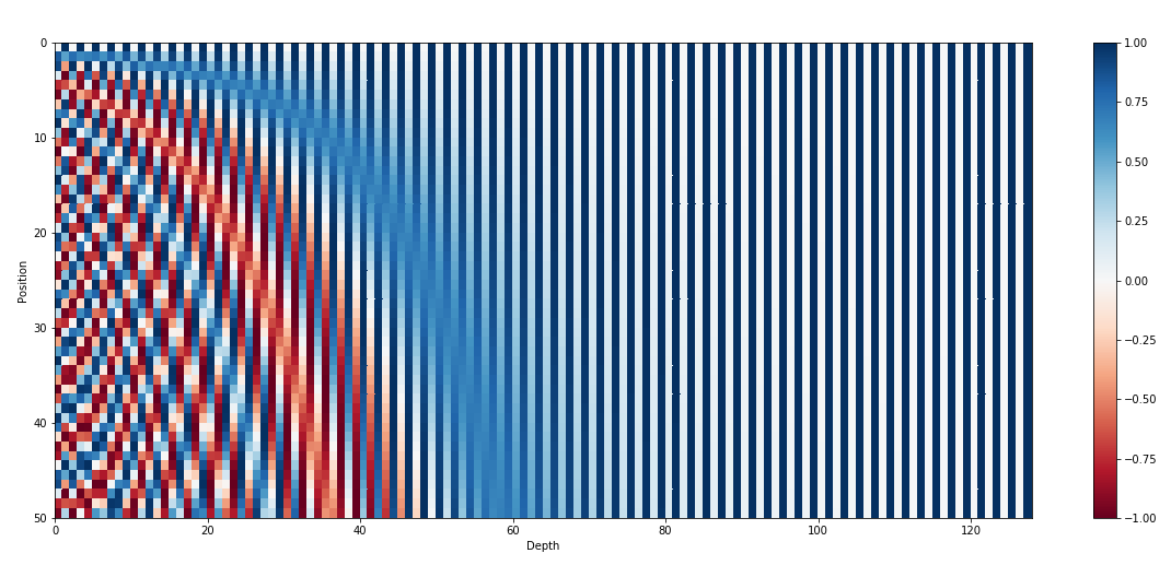
- Remarks:
- by giving positional encodings the same dimension as word embeddings, we can sum them together
- most positional information is encoded in the first dimensions, so summing them with word embeddings enable the model to “let” the first dimensions free of semantics and dedicate them to positions.
- Challenge: long-context
Multi-head self-attention
- several attentions in parallel
- concat outputs after self-att
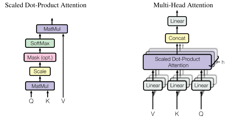
Normalisation
- Add a normalization after self-attention
- parametric center+scale 1 vec across dimensions
- keep gradients small (cf arxiv.org/pdf/2002.04745)
MLP = feed forward
- Add another MLP to store/inject knowledge
- Add residual connections: smooth loss landscape
Layer
- Stack this block \(N\) times
- Gives time to reason = execution steps of a program
- Enables redundancy: Mechanistic interpretability:
- developped by Anthropic AI
- multiple/concurrent circuits
Encoder-decoder
- The transformer is designed for Seq2Seq
- So it contains both an encoder and decoder
- Same approach for decoder
- with cross-attention from encoder to decoder matching layers
- with masks to prevent decoder from looking at words \(t+1, t+2\dots\) when predicting \(t\)
- GPT family: only the decoder stack
- BERT family: only the encoder stack (+ classifier on top)
- T5, BART family: enc-dec
- pure encoders (BERT) have been superseded by enc-dec (T5)
- because T5 learns multiple tasks at once, vs. 1 task for BERT
- advantage of denoising loss decreases with scale
- denoising loss are less efficient than next-token prediction => largest LLMs are all decoders
- Implementation details of the transformer:
- great resource:
- see The annotated transformer
Inductive bias of transformer
- Assume discrete inputs (tokens)
- All positions in sentence have equal importance
- Relates tokens based on similarities / content
- 2 major composants with different roles:
- self-att focuses on relations
- MLP inject knowledge
- Solve limitations of previous models
- No bottleneck of information (as in ConvNet, RNN, seq2seq…)
- No preference for “recent tokens” (as in RNN)
- No constraints of locality (as in CNN)
- … but “lost in the middle” effect
- after learning, transformer can be viewed as a semi-Turing Machine:
- proof that transformer learns in context with gradient descent
- proof that Transformers Learn Higher-Order Optimization Methods for In-Context Learning
- They learn exponentially better learning algorithms than SGD, apparently similar to Iterative Newton’s method
- another proof that it can apply temporal difference (RL algo)
- deep learning models learn algorithms to compress information
Desirable properties
- Can scale
- Can “absorb” huge datasets
- Can “compress” information ==> generalize
- Store facts, but also all types of knowledge: algorithms…
- Can learn in-context
- They can reason along 2 paths:
- depth = nb of layers
- time = stack again above the grown sequence
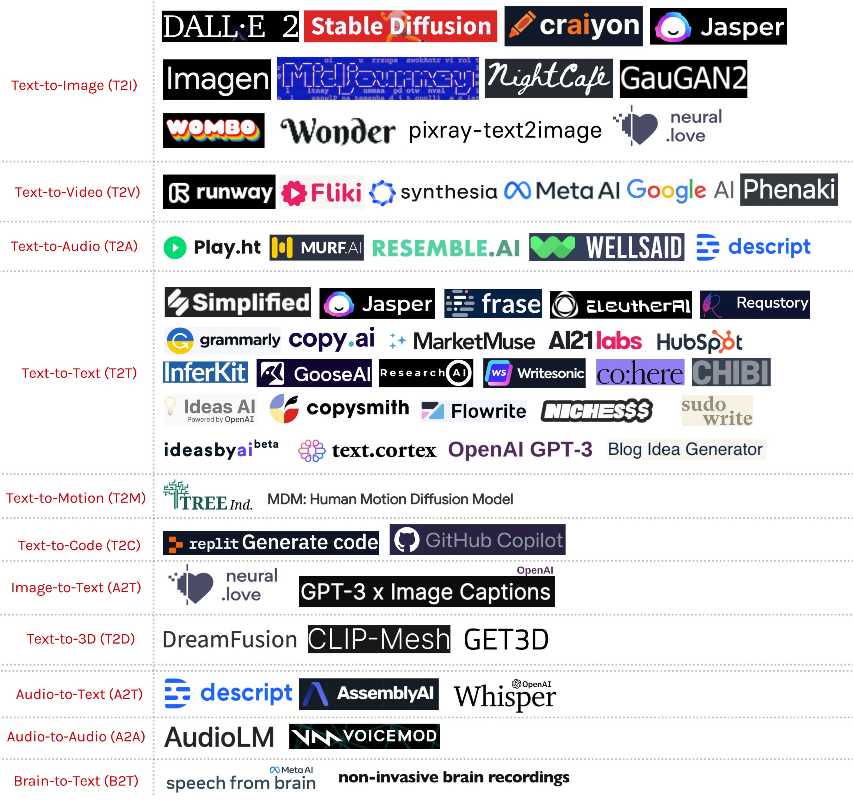
- Transformers have replaced other models in many modalites:
- Image: token = small piece of image
- Audio: token = small segment of sound
- Video, code, DNA…
Terminology
- Activations: output of each layer
- Embeddings:
- context-indep embeddings at the first layer
- context-dep embeddings at the last layer
- Latent representations: all activations
- head:
- converts top embeddings: LM-head, Classification-head, Seq-head, Regression-head…
- Att-head: process part of the activations
Tokenization
- A token is actually computed on a corpus. Most famous tokenizers: SentencePiece, WordPiece, Byte-Pair Encoding (BPE).
- BPE:
- tokenize texts into words, count occurrences
- split words into chars: “cat”,10 -> “c” “a” “t”, 10
- merge most frequent pair, e.g., (“a”,“t”) -> (“at”)
- repeat last step
Tokenizer quality
- Choosing the right tokenization is important:
- More tokens -> large embedding matrix
- Longer tokens have less training instances, but better captures semantics
- Longer tokens -> smaller context length
- Tokens must represent well the target texts
- Multilingual LLMs: language specific tokens
- Evaluation with: (lower is better)
- fertility = avg nb of subwords per word
- % of splitted words
BERT tok fertility:
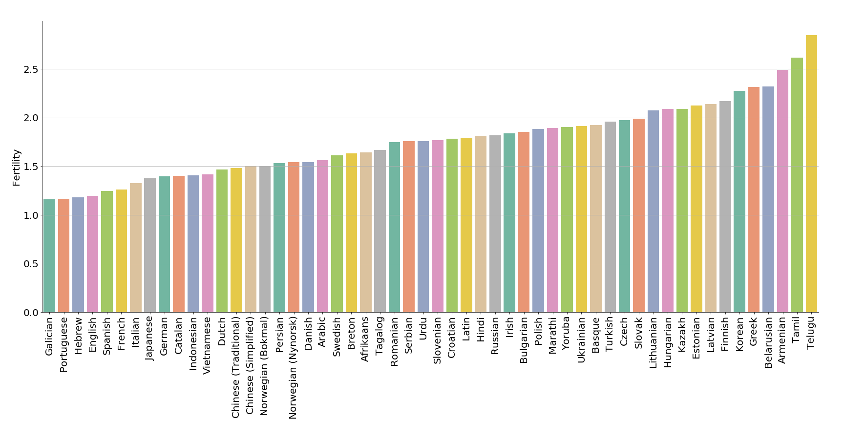
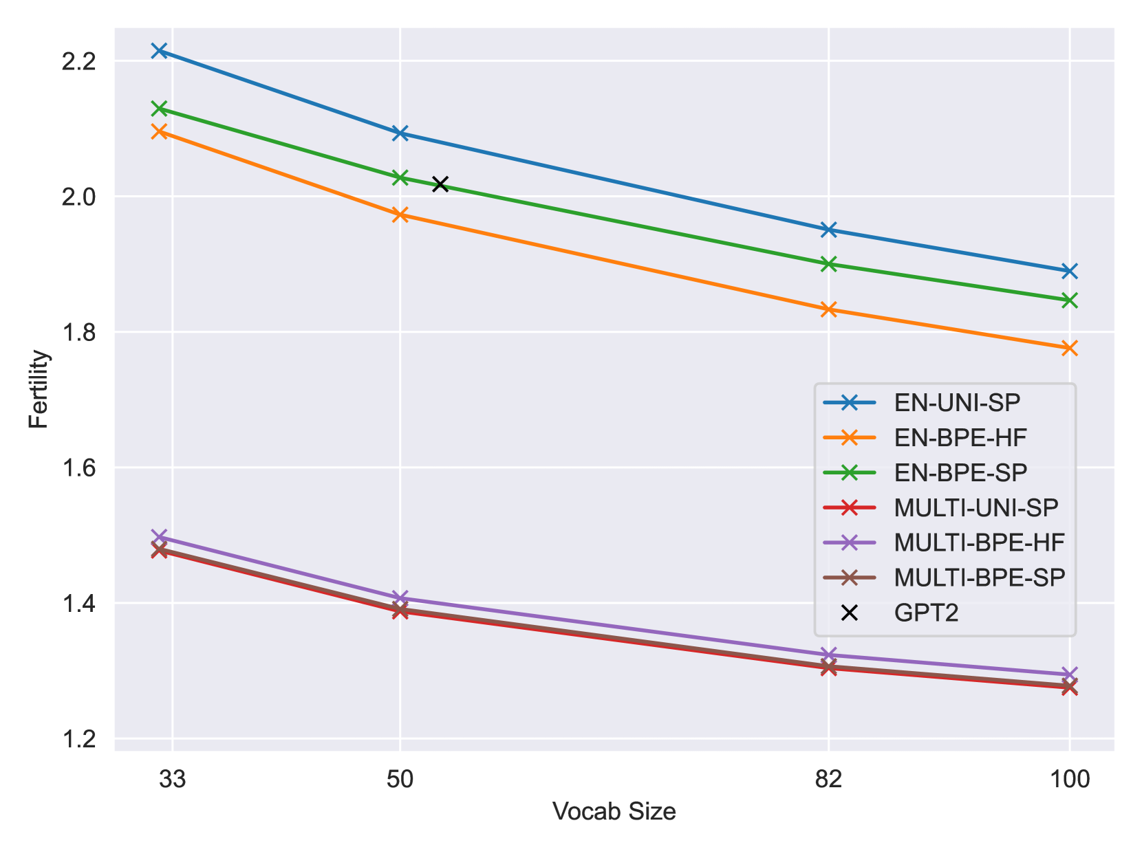
- Fertility smaller (closer to 1) shows that the tokens represent well the language/corpus.
- Comparison of tokenizers:
Tokenizer impact on training costs
- Smaller fertility leads to smaller training costs, but there’s a compromise (Narayanan, 2021):
\[C=96Flh^2\left( 1+\frac s {6h} + \frac V {16lh} \right)\]
\(s=\) sent length, \(l=\) layers, \(h=\) hidden size, \(V=\) vocabulary, \(F=\) fertility, \(C=\) cost per word of 1 forward-backward.
Tokenizer design
- Challenge: repeated long seqs may give 1 token!
- Deduplication during preprocessing
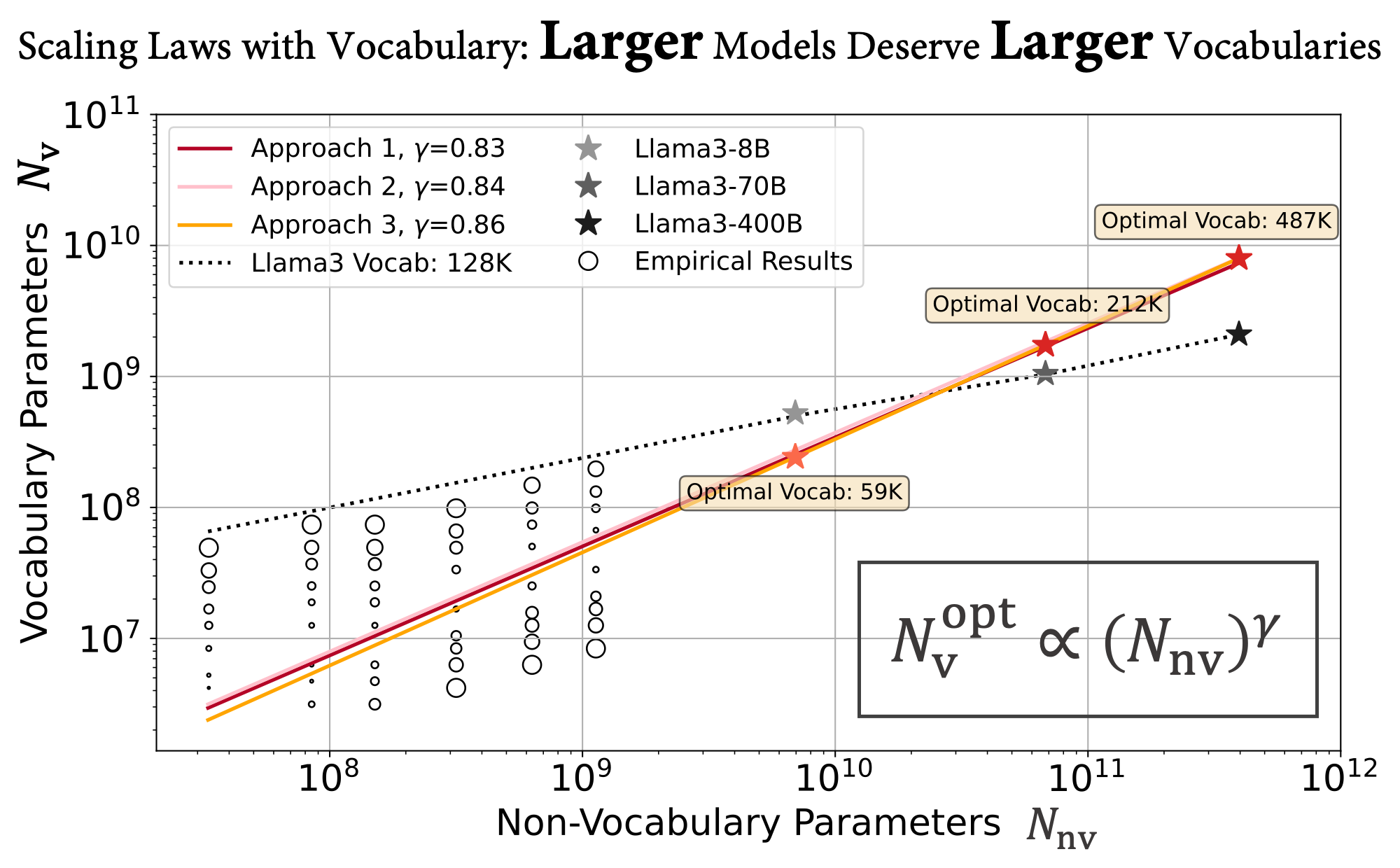
- Best practices: vocab size:
- Bloom: 256k
- GPT3.5: 52k
- Falcon: 64k
- Llama2: 32k
- GPT4: 100k
- Llama3: 128k
- Qwen2: 150k
- Gemma: 256k
Contrastive training
Retrieval Augmented Generation
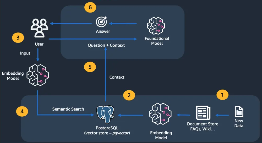
- Embedding model
- encodes all document “paragraphs”
- Vector store
- stores all “paragraph” embeddings
- Retriever
- Finds 10 most relevant “paragraphs” to question Q
- LLM
- Generates answer given 10 retrieved paragraphs and Q
- Embedding model is from the SBERT family
- LLM is from the GPT family
- Both are transformers!
What is the difference between the embedding model and the LLM? Why not a single LLM?
- Embedder:
- role: generate an embedding that represents the semantics of the paragraph
- small: its task is relatively easy: finding the semantically closest paragraphs to the question;
- fast: there may be many paragraphs to encode
- size < 1b parameters (usually)
- LLM:
- role: understand context and answer question
- large: its task requires lots of knowledge and reasoning
- size > 7b parameters (usually)
- Embedders and LLM ~= transformers
If both embedders and LLM are transformers, what is their difference? (Think training)
- Goal of embedders = compute 1 semantic embedding vector
- Training: masked language modeling, contrastive
- Goal of LLM = generate answer
- Training: causal language modeling
- Masked Language Modeling (MLM) objective:
- mask a random word in the input sentence and ask the model to predict it
- Causal Language Modeling (LM) objective:
- remove the end of the input sentence and ask the model to predict the next word
- In both cases (MLM and LM):
- we get the embedding \(z \in R^d\) at the output of the transformer
- we predict the target word \(\hat w \in V\) from \(z\) through a linear classifier:
- logits = \(y\in R^{|V|}\) = scores for each possible word: \(y = Ez\) with \(E\in R^{|V|\times d}\) \[\hat w = \arg\max_{1\leq i\leq |V|} y_i\]
- So why is \(z\) better for semantic search with MLM than with LM?
- LM: the final \(z\) only contains information about the next word
- so not much information about the input sentence itself!
- = GPT family
- MLM: we must be able to reconstruct any word from \(z\)
- so info about the input sentence passes to the top
- = BERT family
TP: RAG
- Implement a RAG using only python and ollama
- Several libraries enable implement RAG: transformers, sentence-transformers, llamaindex, langchain, haystack, DSPy…
- We’ll use ollama, which main advantages are:
- Designed to be ready-to-use & easy-to-learn
- Designed to run locally on laptops
- It is fast, uses 4-bits models by default, supports embeddings and LLMs
- Data
- we’ll use headlines scrapped from France Info in 2024
- The goal is to be able to query the LLM about recent news in French and with the French point of view
- Embedding model:
- Embedding model: must support French, be lightweight
- See the HF MTEB leaderboard
- We’ll use the paraphrase-multilingual-minilm
- LLM model:
- Must be good in French, and lightweight
- We’ll use Qwen2.5-7b quantized in 4 bits (reqs: RAM > 8GB)
- Here’s a code you can copy/paste in your python environment
import ollama
from numpy.linalg import norm
import numpy as np

# first download data: wget https://olki.loria.fr/cerisara/lexres/frnews.txt

# embedding model:
em="nextfire/paraphrase-multilingual-minilm"

def find_most_similar(needle, haystack):
    needle_norm = norm(needle)
    similarity_scores = [
        np.dot(needle, item) / (needle_norm * norm(item)) for item in haystack
    ]
    print("debug",similarity_scores)
    return sorted(zip(similarity_scores, range(len(haystack))), reverse=True)


SYSTEM_PROMPT = """You are a helpful reading assistant who answers questions
        based on snippets of text provided in context. Answer only using the context provided,
        being as concise as possible. If you're unsure, just say that you don't know.
        Context:
    """

with open("frnews.txt","r") as f: lines = f.readlines()
bdd = []
for i,l in enumerate(lines):
    if i>=50: break
    # see https://sbert.net/examples/applications/computing-embeddings/README.html
    embeddings = ollama.embeddings(model=em, prompt=l)["embedding"]
    bdd.append(embeddings)
print("bdd built")

q="Dans quelle ville y a-t-il eu des canicules ?\n"
prompt_embedding = ollama.embeddings(model=em, prompt=q)["embedding"]
most_similar_chunks = find_most_similar(prompt_embedding, bdd)[:1]
print("retrieved:",most_similar_chunks,lines[most_similar_chunks[0][1]])

response = ollama.chat(
        model="qwen2.5",
        messages=[
            {
                "role": "system",
                "content": SYSTEM_PROMPT
                + "\n".join([lines[x[1]] for x in most_similar_chunks]),
            },
            {"role": "user", "content": q},
        ],
    )
print("\n\n")
print(response["message"]["content"])

# see https://decoder.sh/videos/rag-from-the-ground-up-with-python-and-ollama- TODO:
- run the code and check that it’s working fine
- try to increase the size of the vector-DB (50 for now) and optionally store the vectors on disk so that they don’t have to be recomputed if it’s too slow
- (opt) Find another domain than FR news with documents (often PDFs, but they need to be converted into text) and adapt this code for this other domain
- Notes:
- when the database becomes large, you must use specialized vector databases and/or specialized search library like Meta FAISS.
- in practice, most common issues with RAG come from the retriever, which does not get the “most relevant” documents;
- real RAG applications require adapting the retriever to business concepts: e.g., with FR news, the “date” should be a primary key to retrieve relevant context and should be handled separately.
- many enhancements of this basic RAG pipeline have been proposed.
- If you ask your RAG: “How many fires in 2024?”
- Assume there were 50 fires: why can’t your RAG answer correctly?
- Assume you can put 60 documents in context: can your RAG answer correctly?
- How could you improve your RAG to answer these kinds of questions?
- You have seen MLM and LM training
- But RAG embedders \(\neq\) vanilla BERT
- Embedders \(\in\) SBERT (sentence-BERT) family
- continue training BERT contrastively
- Why vanilla BERT are not good enough embedders?
- Because vanilla BERT produces an embedding space where paraphrases are not always close together
- Contrastive learning is a training objective to:
- Control the “shape” of the embedding space
- align multimodal embeddings
BERT is not good enough: similar words are not close enough in its embedding space.
def: embedding space = vector (\(\in R^d\)) that BERT outputs for each word in the sentence. If you pass into BERT every English sentences, you obtain the full embedding space.
Let’s verify!
Practice: plot BERT embeddings
- Download distilBERT, compute the embeddings for a few sentences with paraphrases or not
- Compute distances and project embeddings in 2D with t-SNE to plot them
- Study the proximity (or not) of paraphrases
    'The table is made of wood'
    'The excel table is large'
    'The digits array can be compressed'
    'The plastic chair is blue'
Hints below…
- SNE
- \(p_{j|i}=\) proba that point i pick j as neighbor (computed from distance btw points)
- \(q_{j|i}=\) same proba in the lower dim
- minimize KL-div btw both probs
pip install transformers[torch]- Print the embeddings:
from transformers import AutoTokenizer, AutoModel, pipeline
model = AutoModel.from_pretrained('distilbert-base-uncased')
tokenizer = AutoTokenizer.from_pretrained('distilbert-base-uncased')
nlp = pipeline('feature-extraction', model=model, tokenizer=tokenizer)
s = 'Do you like cakes ?'
features = nlp(s)
print([features[0][i][:2] for i in range(len(features[0]))])- Look at the input tokens:
inputs = tokenizer.encode_plus(s, add_special_tokens=True, return_tensors="pt")
input_ids = inputs["input_ids"].tolist()[0]
text_tokens = tokenizer.convert_ids_to_tokens(input_ids)
print(text_tokens)- Compute the distance between 2 embedding vectors:
from sklearn.metrics.pairwise import cosine_similarity
print(cosine_similarity(v1,v2))- project a distance matrix:
from sklearn import manifold
tsne = manifold.TSNE(n_components=2, metric="precomputed", perplexity=2)
res = tsne.fit(m)- plot a set of 2D points:
import matplotlib.pyplot as plt
plt.scatter( coords[:, 0], coords[:, 1], marker = 'o')
plt.show()
Contrastive objective
- Compute emb for sent A and B; when sentences are paraphrase, minimize \(|s_A-s_B|\); when they’re different, maximize it.
- See also metric learning, siamese networks, ranking loss
- This enables to control / shape the embedding space the way we want
- used for:
- Pretrained Dense Retrieval in RAG
- multimodal models (CLIP)
Contrastive losses
- pair-wise loss:
\[L=\biggl\{\begin{matrix} d(s_A,s_B) & if~~Positive Pair\\ \max(0,m-d(s_A,s_B)) & if~~Negative Pair \end{matrix}\]
- triplet loss: \(L=\max(d(s_A,s_P) - d(s_A,s_N) + \epsilon, 0)\)
- gives better embedding space
- InfoNCE: \(N\) batches with \(M\) samples: 1 positive (0) and \(M-1\) negative (\(1\dots M-1\)):
\[L= - \frac 1 N \sum_{i=1}^N \log \frac{e^{sim(s_{A_i},s_0)}}{\frac 1 M \sum_{j=0}^{M} e^{sim(s_{A_i},s_j)}}\]
- Main challenge: how to sample negative examples?
- easy neg: too far from pos, nothing is learnt
- hard neg: too close to pos, instable learning
- semi-hard negatives!
Once an embedding space is trained, how can you use it to directly perform instance-based classification?
- refs: Lilan Weng blog
- You compare the unknown embedding with all known (training) embeddings, and assign it the class of the closest known
- important to understand this method!
- Real-life examples of embeddings use: Pinterest, Youtube…
Practice: plot BGE
- plot the distance matrix between sentences when computed with BAAI/bge-base-en-v1.5 instead of BERT, compare.
- Better comparison:
- Use a corpus annotated with topics instead of a few sentences:
from datasets import load_dataset
ds = load_dataset("fancyzhx/ag_news", split='test')
Ranking vs. Cross-ent loss
(see github blog)
- Train ConvNet on MNIST with 10-class cross-entropy loss
- No need of tSNE when training: directly define a 2D-embedding space by adding a final linear layer to the model
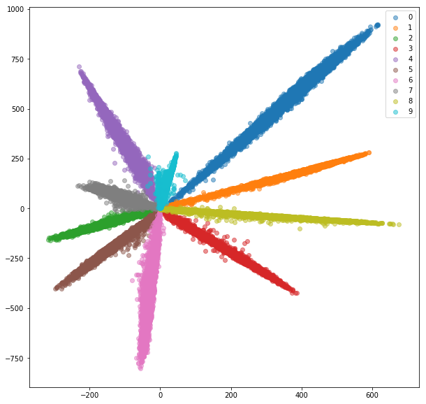
- Distance btw classes not good
- Train a siamese net
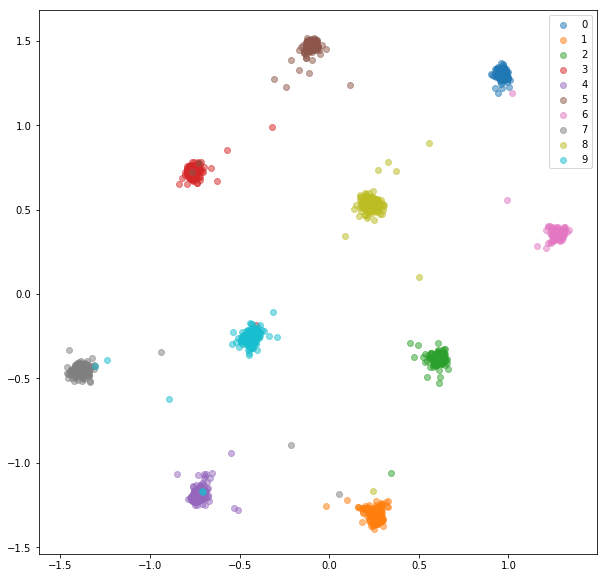
- Distance btw classes are good
- Train a triplet net
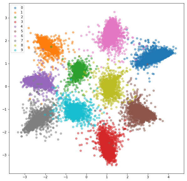
- Didn’t train for same-class embed. get closer, but trained for same class embed. to be closer than inter-class embed.
Other advantages of ranking loss
- Cross-Ent loss not robust to noisy labels
- Many classes are costly with softmax
- Meaningful dist btw embeddings is desirable (S-BERT)
Practice: train with triplet loss
- Goal: train an embedding model with triplet loss
- Until now, you’ve only used already trained embedding models
- Synthetic data:
- scalar input, 2 classes \(c\in \{0,1\}\)
- \(x|c \sim N(\mu_c,\sigma_c=0.1)\)
- Embedding dim = 5
- lightning = pytorch library that
- automates cpu/gpu runtime
- simplifies training loop
- generates tensorboard logs
- pytorch lightning in practice:
- replace and extend nn.Module:
import pytorch_lightning as pl

class Mod(pl.LightningModule):
    def __init__(self):
        super().__init__()
        self.W = torch.nn.Linear(1,5)

    def configure_optimizers(self):
        opt = torch.optim.AdamW(self.parameters(), lr = 1e-3)
        return opt

    def training_step(self, batch, batch_idx):
        anc, pos, neg = batch
        ea = self.W(anc)
        ep = self.W(pos)
        en = self.W(neg)
        dp = torch.nn.functional.triplet_margin_loss(ea,ep,en)
        self.log("train_loss", dp, on_step=False, on_epoch=True)
return dp- you need a dataset that generates anchors/pos/neg:
class TripDS(torch.utils.data.Dataset):
    def __init__(self):
        super().__init__()

    def __len__(self):
        return 1000

    def __getitem__(self,i):
        if i%2==0:
            # pair: on sample une ancre from class 1
            z = random.randint(0,1)
            if z==0: xa = torch.randn(1)/10.-0.5
            else: xa = torch.randn(1)/10.+1.5
            z = random.randint(0,1)
            if z==0: xp = torch.randn(1)/10.-0.5
            else: xp = torch.randn(1)/10.+1.5
            xn = torch.randn(1)/10.+0.5
        else:
            # impair: on sample une ancre from class 2
            xa = torch.randn(1)/10.+0.5
            xp = torch.randn(1)/10.+0.5
            z = random.randint(0,1)
            if z==0: xn = torch.randn(1)/10.-0.5
            else: xn = torch.randn(1)/10.+1.5
return xa,xp,xn- Train:
traindata = TripDS()
trainloader = torch.utils.data.DataLoader(traindata, batch_size=1, shuffle=False)
mod = Mod()
logger = pl.loggers.TensorBoardLogger(save_dir="logs/", flush_secs=1)
trainer = pl.Trainer(limit_train_batches=1.0, max_epochs=1000, log_every_n_steps=1,logger=logger)
trainer.fit(model=mod, train_dataloaders=trainloader)- TODO:
- run this training and observe the logs with:
tensorboard --logdir=lightning_logs/- does it converge?
- adap this code so that the model is a 2 layer MLP, the output embedding space is 2D, and plot 100 points with matplotlib before and after training
CLIP
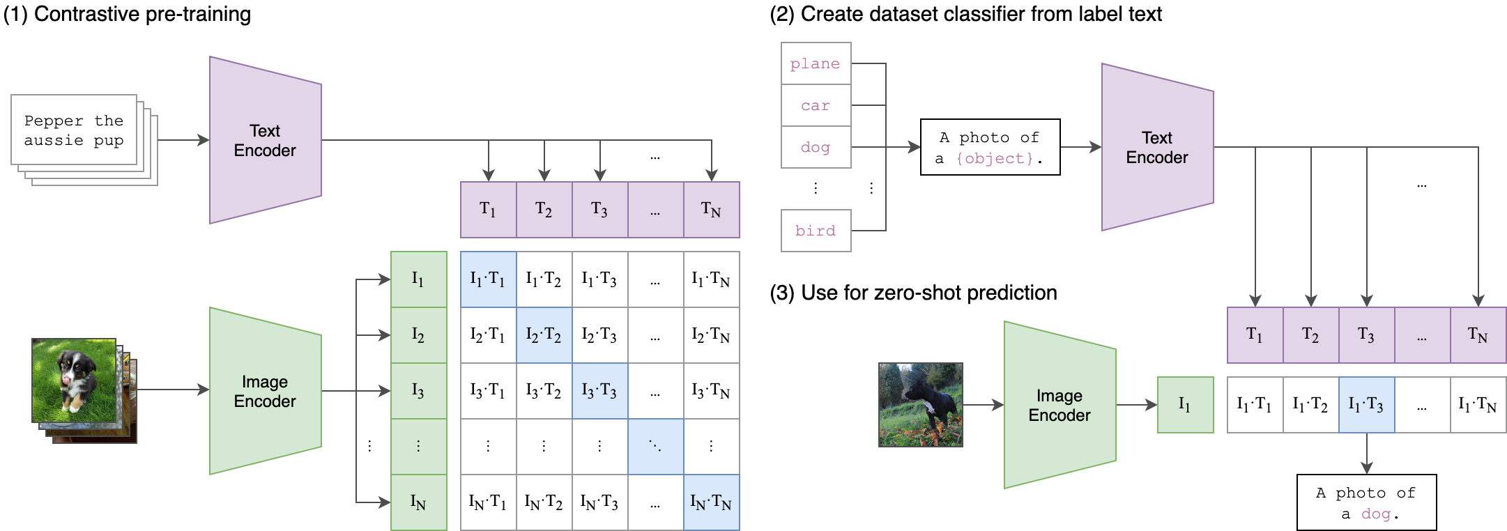
- CLIP is a model that builds a joint text/image embedding space
- uses 2 transformers, resp. for image and text + cosine dist
- It is trained with a ranking loss: multi-class N-pair loss
- they show that ranking loss much faster to train
- Given an input image and several texts, it outputs similarity scores
- How to use it:
from transformers import CLIPProcessor, CLIPModel, CLIPTokenizer
from PIL import Image

model = CLIPModel.from_pretrained("openai/clip-vit-base-patch32")
processor = CLIPProcessor.from_pretrained("openai/clip-vit-base-patch32")
image = Image.open("difftrain.png")
inputs = processor(text=["a rabbit","a curve","a chair"], images=image, return_tensors="pt", padding=True)
outputs = model(**inputs)
logits_per_image = outputs.logits_per_image  # this is the image-text similarity score
probs = logits_per_image.softmax(dim=1)  # we can take the softmax to get the label probabilities
Wrap-up
- You can define your own distance between embeddings with contrastive learning
- For generation, use a large LLM (trained on next word prediction)
- RAG is the first method to try when you have to deal with company’s documents
- … but RAG is not magic, retrieval requires a lot of work specific to each case
Embedding distances:
- dot product
- Cosine similarity: \(sim(w,u)=\frac {u \cdot v}{||u||~~||v||}\)
Other embeddings: One-hot encoding
- Orthogonal normed vectors: all words are equal
- Can be processed with matrix algebra
- But high dim and fixed vocabulary
- highly sub-optimal (symetries)
Other embeddings: Probabilistic models
- Blei, Ng and Jordan, 2003
- Latent Dirichlet Allocation: learn the distributions
- P(word | topic) and P(topic | document)
- P(topic | document) == document embedding
- Can infer P(topic | word) == (explainable) word embedding!
Other embeddings: Vector space models
- Implementation of distributional hypothesis: “You shall know a word by the company it keeps” [Firth, 1957]
- Word embedding = vector of nb of occurrences of word in each document
- == term-document matrix
- But high dim, noisy
- Methods to “compress” the matrix:
- Latent Semantic Analysis (LSA) (1990), HAL (1997), BEAGLE (2007), Glove (2014)
- Special case: random indexing (2006)
Other embeddings: Random indexing
Johnson-Lindenstrauss lemma: projection into random high-dim subspace approx. preserves distances
Init: each word \(w\) is assigned an index random sparse vector \(I_w\), and a context null vector \(C_w\).
For every \(u\) in the context of \(w\): \(C_w \leftarrow C_w + I_u\)
Very fast
Incremental
Other embeddings: Neural static embeddings
- “word embedding” proposed by Bengio in 2003
- Collobert embeddings (2008): trained on NLP tasks
- Word-to-vec (Mikolov, 2013): trained to predict context
- FastText
- Problems: OOV? Polysemy? MWE?…
Other embeddings: Sentence embeddings
- NN-LM (Bengio): \(s = P(w_t|w_1,\dots,w_{t-1})\)
- Averaging word embeddings: \(s=\frac 1 T \sum_t w_t\)
- Doc2Vec (Mikolov): Avg with paragraph vector
- Skip-thought: generates context sentences
- Quick-thought: classifies candidates context sentences
- InferSent: trained on NLI
- Universal sentence encoder (Google, 2018): Deep Averaging Network
- Sentence BERT (2019)
Tools for embeddings
- Gensim: LDA, LSI, TFIDF, W2V, Doc2Vec…
- SpaCy: BERT, XLNET…
- FastText: multilingual, fast and large W2V
- SentEval: Skipthought, UnivSE, InferSent
- HF Transformers: includes all
LLM adaptation
- First: LLMs are pretrained (not your business)
- Second: you want to use an LLM for your task:
- Is the pretrained LLM good enough?
- If not:
- can I train a small model on my task’s data?
- how can I adapt it = make it better for my task?
Pretrained LLM compromise
- Training an LLM is fundamentally a compromise:
- training data mix: % code/FR/EN…
- text styles: twitter/books/PhD…
- Pretraining data mix defines where the LLM excels
- Finetuning modifies this equilibrum to our need
- The art of pretraining:
- finding the balance that fits most target users’ expectation
- finding the balance that maximizes the LLM’s capacities + adaptability
- e.g., pretraining only on medical data gives lower performance even in healthcare, because of limited data size and lack of variety.
- But for many specialized tasks, pretrained LLM does not give the best performance:
- Finetuning adapts this compromise
Is it possible to get the ideal pretrained LLM for everything?
- more data is always best (even for SmolLM!)
- So why not training the largest LLM ever on all data and use it everywhere?
- Usage cost
- Obsolescence
- Data bottleneck
- So far, not good enough for most cases!
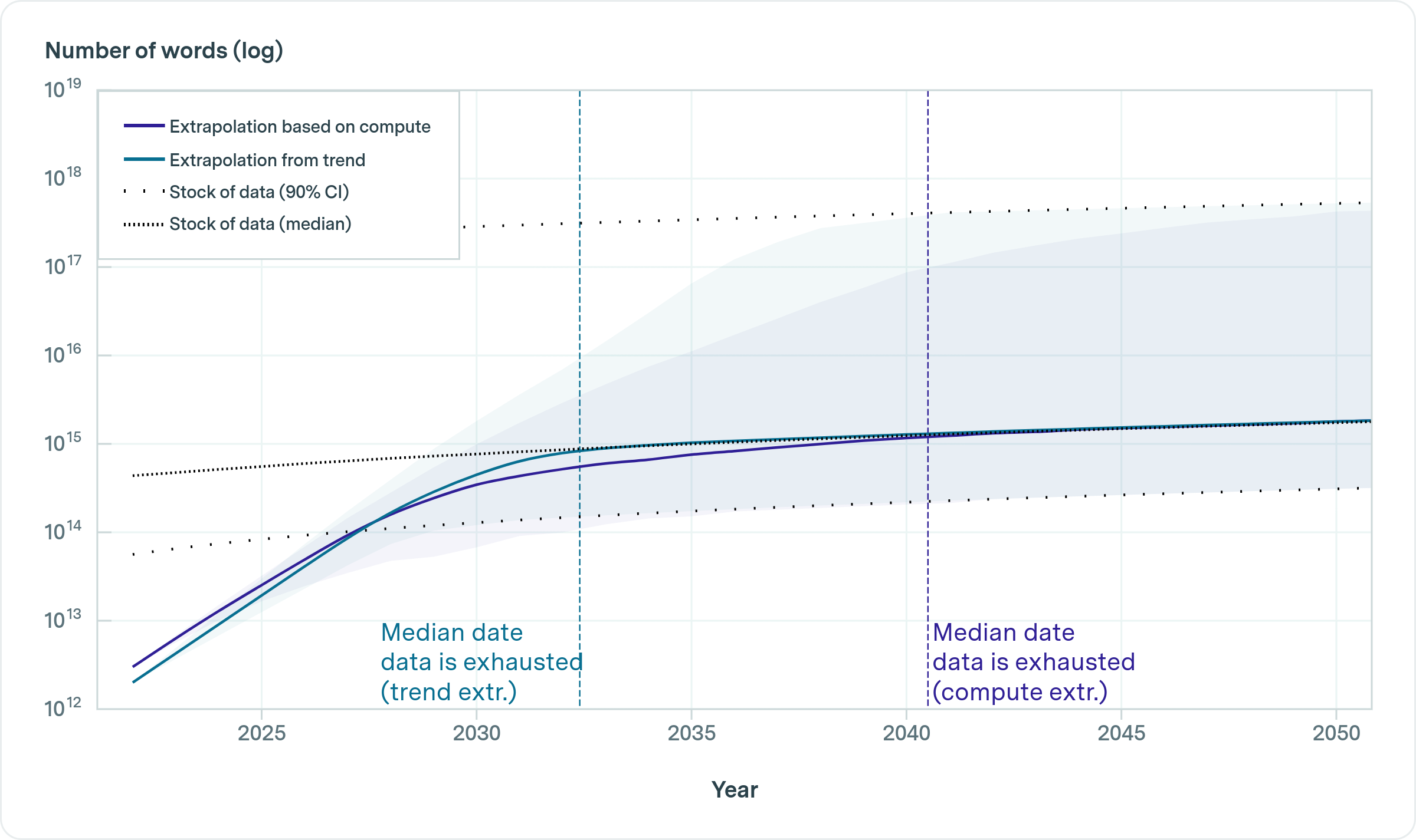
Main options to adapt
- First try the cheapest options:
- Prompt engineering
- LLM agents
- small model on your data (may not be recommended)
- AI as features computer
- PEFT
- Finetuning
- Why not just training a small model from scratch on the target domain?
- Transfer learning: we expect to transfer capabilities from the generic AI to get a better target model
- Small data: we often don’t have enough domain data to train a small model from scratch, but specializing the generic AI model usually requires few data
- LLM agents
- LLM controls (part of) the data flow
- Tools/Function calling: LLMs call APIs
- Code generation: LLMs generate (and execute) code
- Planning: LLMs plan actions and orchestrate their execution
- AI as features computer
- AI is used as a black box to represent input sentences/speech/images/…
- Each input is passed to AI model that outputs an embedding
- This embedding is used as input to the rest of the software system
- AI as features computer can be viewed as special case of finetuning:
- X \(\rightarrow\) AI \(\rightarrow\) Embeddings \(\rightarrow\) Classifier
- The AI module may be kept frozen
- But the classifier must be trained on data:
- It’s often best to further train backward into the AI model, but it’s much more costly
Motivation for PEFT
- PEFT = Parameter-Efficient Fine-Tuning
- It’s just finetuning, but cost-effective:
- only few parameters are finetuned
- cheaper to train
- cheaper to distribute
When do we need finetuning?
- Improve accuracy, adapt LLM behaviour
- Finetuning use cases:
- Follow instructions, chat…
- Align with user preferences
- Adapt to domain: healthcare, finance…
- Improve on a target task
Finetuning
- Finetuning = continue training the AI model on domain-specific data
- The training objective may change (e.g., new image classification)
- Or it may stay the same as pretraining (e.g., language modeling)
- Pretraining \(\rightarrow\) Foundation models
- Finetuning \(\rightarrow\) Domain-specific models
- Stochastic Gradient Descent (SGD) (part1):
- You need a training corpus \(C = \{x_i,y_i\}_{1\leq i\leq N}\)
- Initialize the model’s parameters randomly: \(\theta_i \sim \mathcal{N}(0,\mu,\Sigma)\)
- Forward pass: sample one example \(x_i \sim \mathcal{U}(C)\) and predict its output: \(\hat y=f_{\theta}(x_i)\)
- Compute the loss = error made by the model: \[l(\hat y, y_i) = ||\hat y - y_i||^2\]
- Stochastic Gradient Descent (SGD) (part2):
- Backward pass: compute the gradient of the loss with respect to each parameter: \[\nabla l(\hat y, y_i) = \left[ \frac {\partial l(\hat y, y_i)}{\partial \theta_k}\right]\]
- Update parameters: \(\theta_k \leftarrow \theta_k - \epsilon \frac {\partial l(\hat y, y_i)}{\partial \theta_k}\)
- Iterate from the forward pass
- Backpropagation algorithm (for the backward pass):
- Compute the derivative of the loss wrt the output: \(\frac {\partial l(\hat y, y_i)}{\partial \theta_T}\)
- Use the chain rule to deduce the derivative of the loss after the op just before: \[\frac {\partial l(\hat y, y_i)}{\partial \theta_{T-1}} = \frac {\partial l(\hat y, y_i)}{\partial \theta_T} \times \frac {\partial \theta_T}{\partial \theta_{T-1}}\]
- Only requires to know the analytic derivative of each op individually
- Iterate back to the input of the model
Train with HF-transformers
With HF transformers lib: classification
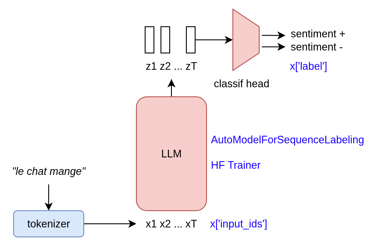
(ask ChatGPT for code samples)
With HF transformers lib: auto-regressive training
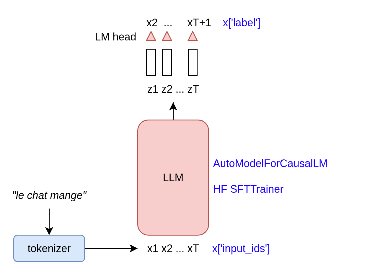
With Pytorch (low-level): training loop
- Pseudo-code:
opt = torch.optim.Adam(model.parameters(), lr=0.001)
floss = torch.nn.CrossEntropyLoss()
x=tokenizer("le chat dort")
for ep in range(epochs):
  opt.zero_grad()
  y = model(x)
  loss = floss(y,labels)
  loss.backward()
opt.step()- Works for classification, auto-regressive: only labels change
- So finetuning is just continued pretraining?
- Yes:
- Same training algorithm (SGD)
- No:
- different hyperparms (larger learning rate…)
- different type of data
- higher quality, focused on task
- far less training data, so much cheaper
- not the same objective:
- adaptation to domain/style/task/language…
- So finetuning is required for many specialized domains:
- enterprise documentations
- medical, finance…
- But it is costly to do for large LLMs:
- collecting, curating, cleaning, formatting data
- tracking training, preventing overfitting, limiting forgetting
- large LLMs require costly hardware to train
- For instance, finetuning LLama3.1-70b requires GPUs with approx. 1TB of VRAM
- = 12x A100-80GB
- Can’t we avoid finetuning at all, but still adapt the LLM to our task?
- Finetuning can be more or less costly:
- just train the classifier on top
- also train the few last layers
- or train 1 middle layer
- or train additional parameters
- or train everything
- …
Which pretrained LLM to finetune?
- Option 1: large LLM
- benefit from best capacities
- fine for not-so-much specialized tasks
- high cost
- Option 2: “small” LLM
- fine for very specialized task
- low cost
- hype: small agent LLMs, smolLM
- larger LLM \(\rightarrow\) less forgetting
Challenges
- Choose pretrained LLM
- Depends on the task and expected performance, robustness…
- Collect quality data
- Finetuning data must be high quality!
- Format data
- Format similar to final task
- FT on raw text may impact instruction following
- Track & prevent overfitting, limit forgetting
- Cost of finetuning may be high
Cost
- Cost of inference << cost of finetuning
- quantization: we don’t know (yet) how to finetune well quantized LLMs; so finetuning requires 16 or 32 bits
- inference: no need to store all activations: compute each layer output from it’s input only
- inference: no need to store gradients, momentum
- Inference can be done with RAM = nb of parameters / 2
- Full finetuning requires RAM = \(11\times\) nb of parameters (according to Eleuther-AI), \(12-20\times\) according to UMass
- 1 parameter byte = +1B (gradient) + 2B (Adam optimizer state: 1st and 2nd gradient moments) (see next slide)
- Can be reduced to \(\simeq 5\times\):
- gradient checkpointing
- special optimizers (1bitAdam, Birder…)
- offloading…
- Adam equations:
- \(m^{(t)} = \beta_1 m^{(t-1)} + (1-\beta_1) \nabla L(\theta^{(t-1)})\)
- \(v^{(t)} = \beta_2 v^{(t-1)} + (1-\beta_2) \left(\nabla L(\theta^{(t-1)})\right)^2\)
- Bias correction:
- \(\hat m^{(t)} = \frac {m^{(t)}}{1-\beta_1}\)
- \(\hat v^{(t)} = \frac {v^{(t)}}{1-\beta_2}\)
- \(\theta^{(t)} = \theta^{(t-1)} - \lambda\frac{\hat m^{(t)}} {\sqrt{\hat v^{(t)}} + \epsilon}\)
- PEFT greatly reduce RAM requirements:
- can keep LLM parameters frozen and quantized (qLoRA)
- store gradients + momentum only in 1% of parameters
- But:
- still need to backpropagate gradients through the whole LLM and save all activations
- with large data, PEFT underperforms full finetuning
VRAM usage
| Method | Bits | 7B | 13B | 30B | 70B | 110B | 8x7B | 8x22B |
|---|---|---|---|---|---|---|---|---|
| Full | 32 | 120GB | 240GB | 600GB | 1200GB | 2000GB | 900GB | 2400GB |
| Full | 16 | 60GB | 120GB | 300GB | 600GB | 900GB | 400GB | 1200GB |
| LoRA/GaLore/BAdam | 16 | 16GB | 32GB | 64GB | 160GB | 240GB | 120GB | 320GB |
| QLoRA | 8 | 10GB | 20GB | 40GB | 80GB | 140GB | 60GB | 160GB |
| QLoRA | 4 | 6GB | 12GB | 24GB | 48GB | 72GB | 30GB | 96GB |
| QLoRA | 2 | 4GB | 8GB | 16GB | 24GB | 48GB | 18GB | 48GB |
Training methods
| Method | data | notes |
|---|---|---|
| Pretraining | >10T | Full training |
| Cont. pretr. | \(\simeq 100\)b | update: PEFT? |
| Finetuning | 1k … 1b | Adapt to task: PEFT |
| Few-Shot learning | < 1k | Guide, help the LLM |
Wrap-up
- With enough compute, prefer full-finetuning
- HF transformer, deepspeed, llama-factory, axolotl…
- With 1 “small” GPU, go for PEFT
- qLoRA…
- Without any GPU: look for alternatives
- Prompting, RAG…
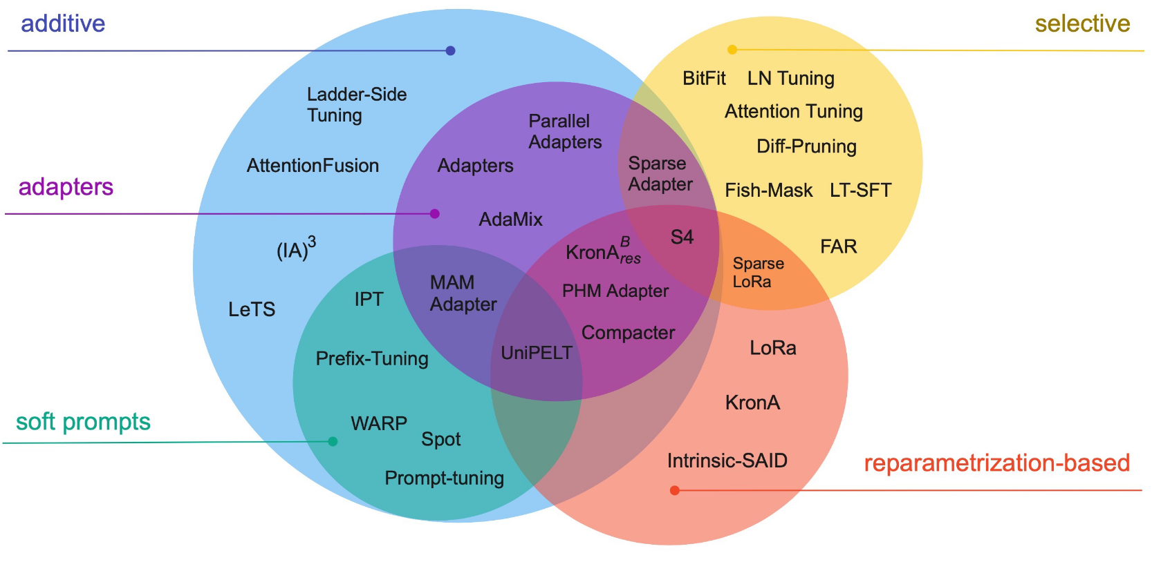
PEFT methods
- do not finetune all of the LLM parameters
- finetune/train a small number of (additional) parameters
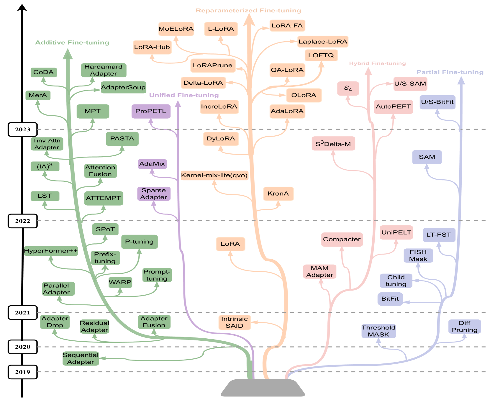
References
We’ll focus on a few
- Additive finetuning: add new parameters
- Adapter-based: sequential adapter
- soft-prompt: prefix tuning
- others: ladder-side-networks
- Partial finetuning: modify existing parameters
- Lottery-ticket sparse finetuning
- Reparameterization finetuning: “reparameterize” weight matrices
- qLoRA
- Hybrid finetuning: combine multiple PEFT
- manually: MAM, compacter, UniPELT
- auto: AutoPEFT, S3Delta-M
- Unified finetuning: unified framework
- AdaMix: MoE of LoRA or adapters
- SparseAdapter: prune adapters
- ProPETL: share masked sub-nets
Sequential adapters
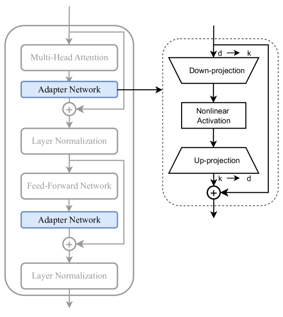
\[X=(RELU(X\cdot W_{down})) \cdot W_{up} + X\]
with
\[W_{down} \in R^{d\times k}~~~~W_{up} \in R^{k\times d}\]
- Advantages:
- Collection of available adapters: AdapterHub
- Drawbacks:
- Full backprop required
- Interesting extensions
- Parallel Adapter (parallel peft > sequential peft)
- CoDA: skip tokens in the main branch, not in the parallel adapter
- Tiny-Attention adapter: uses small attn as adapter
- Adapter Fusion: (see next slide)
- Train multiple adapters, then train fusion
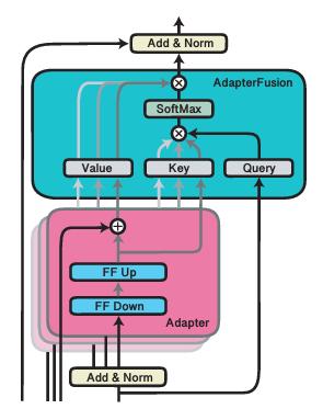
- Related to Adapter merging and LLM merging/LoRA extraction
Prefix tuning
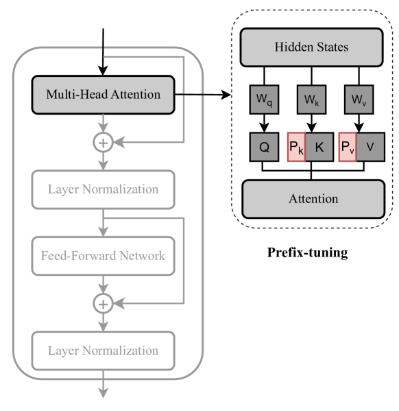
- Concat \(P_k,P_v \in R^{l\times d}\) before \(K,V\) \[head_i = Attn(xW_q^{(i)}, concat(P_k^{(i)},CW_k^{(i)}), concat(P_v^{(i)},CW_v^{(i)})\]
- with \(C=\)context, \(l=\)prefix length
- ICLR22 shows some form of equivalence:

- Advantages:
- More expressive than adapters, as it modifies every attention head
- One of the best PEFT method at very small parameters budget
- Drawbacks:
- Does not benefit from increasing nb of parameters
- Limited to attention head, while adapters may adapt FFN…
- … and adapting FFN is always better
Performance comparison

qLoRA = LoRA + quantized LLM
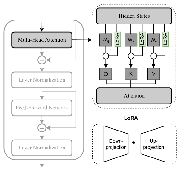
- Advantages:
- de facto standard: supported in nearly all LLM frameworks
- Many extensions, heavily developped, so good performances
- can be easily merged back into the LLM
- Drawbacks:
- Full backprop required
Adapter lib v3
- AdapterHubv3 integrates several family of adapters:
- Bottleneck = sequential
- Compacter = adapter with Kronecker prod to get up/down matrices
- Parallel
- Prefix, Mix-and-Match = combination Parallel + Prefix
- Uniformisation of PEFT functions: add_adapter(), train_adapter()
- heads after adapters: add_classification_head(), add_multiple_choice_head()
- In HF lib, you can pre-load multiple adapters and select one active:
model.add_adapter(lora_config, adapter_name="adapter_1")
model.add_adapter(lora_config, adapter_name="adapter_2")
model.set_adapter("adapter_1")
Ladder-side-networks
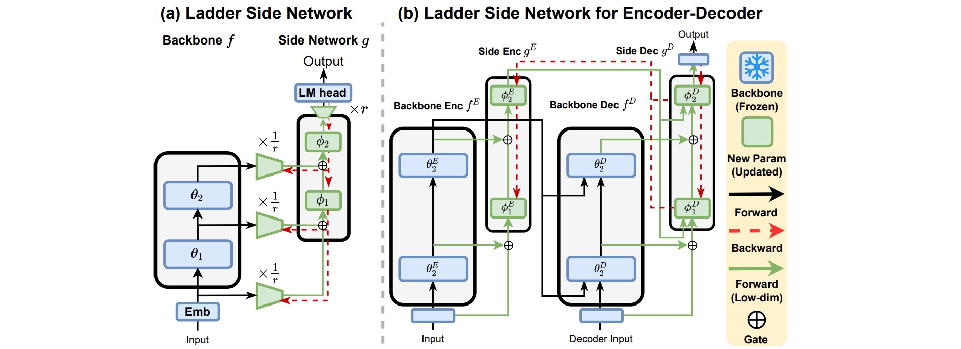
- Advantages:
- Do not backprop in the main LLM!
- Only requires forward passes in the main LLM
- Drawbacks:
- LLM is just a “feature provider” to another model
- \(\simeq\) enhanced “classification/generation head on top”
- Forward pass can be done “layer by layer” with “pipeline parallelism”
- load 1 layer \(L_i\) in RAM
- pass the whole corpus \(y_i=L_i(x_i)\)
- free memory and iterate with \(L_{i+1}\)
- LST: done only once for the whole training session!
- This approach received an outstanding award at ACL’2024:
Partial finetuning
- Add a linear layer on top and train it
- LLM = features provider
- You may further backprop gradients deeper in the top-N LLM layers
- … Or just FT the top-N layers without any additional parameters
- Simple, old-school, it usually works well
- Fill the continuum between full FT and classifier head FT:
- can FT top 10%, 50%, 80% params
- or FT bottom 10%, 50% params
- or FT intermediate layers / params
- or apply a sparse mask?
Lottery-ticket sparse finetuning
- Lottery Ticket Hypothesis:
- Each neural network contains a sub-network (winning ticket) that, if trained again in isolation, matches the performance of the full model.
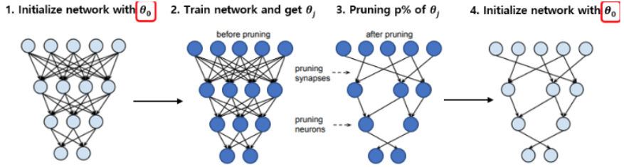
- Advantages:
- Can remove 90% parameters nearly without loss in performances (on image tasks)
- Drawbacks:
- Impossible to find the winning mask without training first the large model
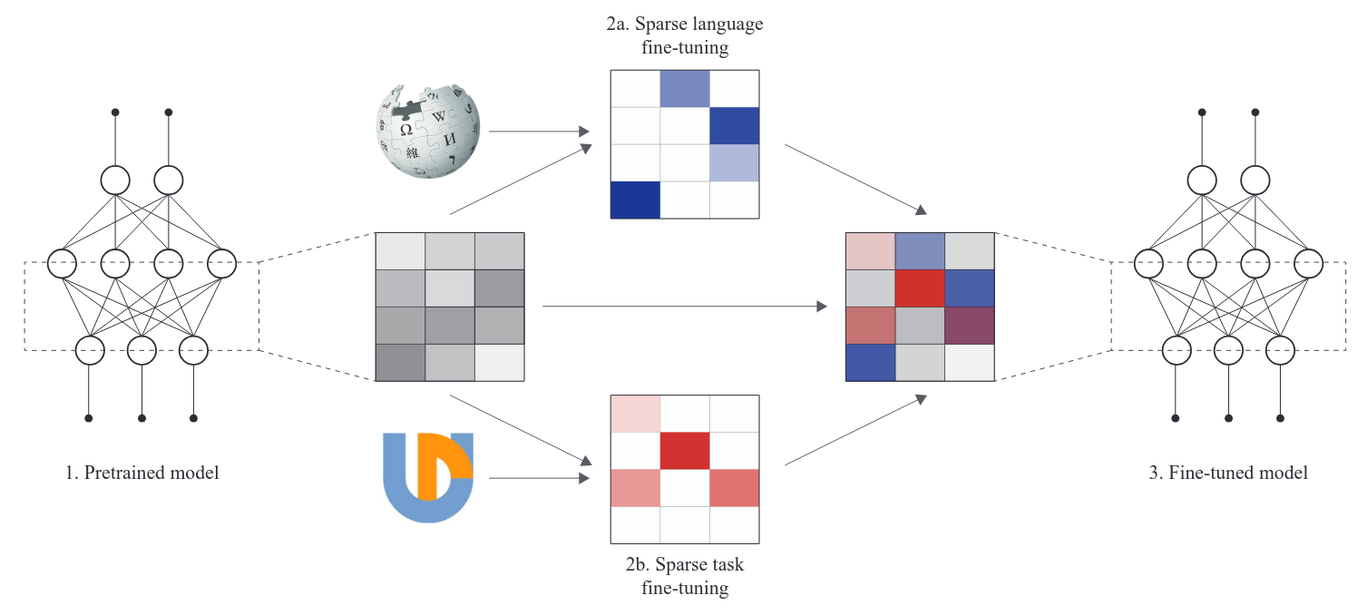
can be applied to sparse FT
FT an LLM on specific task/lang
extract the mask = params that change most
rewind the LLM and re-FT with mask
sparse finetunes can be combined without overlapping!
Wrap-up
- Various PEFT methods:
- Reduce model storage? RAM requirements?
- Require backprop through the LLM?
- Additional inference cost?
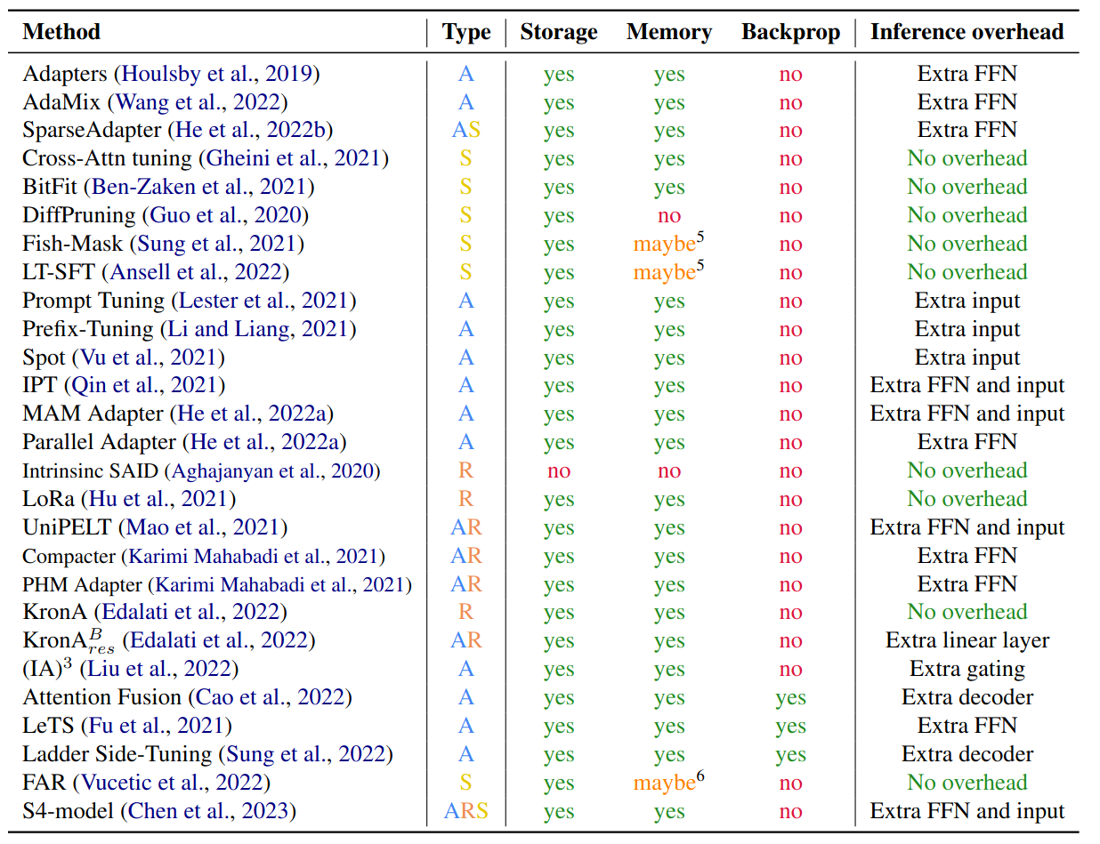
Finetuning (PEFT or full): advantages
- greatly improve performances on a target task, language, domain
- dig knowledge up to the surface, ready to use
- give the LLM desirable capacities: instruction-following, aligned with human preferences…
Finetuning (PEFT or full): drawbacks
- forgetting
- very slow to learn (BitDelta: Your Fine-Tune May Only Be Worth One Bit)
- increase hallucinations
Memorization, forgetting
Pretraining and FT use same basic algorithm (SGD), but the differences in data size lead to differences in training regimes.
- Difference in scale:
- Pretraining ingests trillions of tokens
- Finetuning uses up to millions of tokens
- This leads to differences in regimes / behaviour:
- Pretraining learns new information
- Finetuning exhumes information it already knows
Why such a difference in regimes?
- Because of the way SGD works:
- When it sees one piece of information, it partially stores it in a few parameters
- But not enough to retrieve it later!
- When it sees it again, it accumulates it in its weights \(\rightarrow\) Memorization
- If it never sees it again, it will be overriden \(\rightarrow\) Forgetting
- How many times shall a piece of information be seen?
- cf. Physics of Language Models: Part 3.3, Knowledge Capacity Scaling Laws
- Universal rule:
- an LLM can store up to 2 bit/param of information
- it requires 1000x exposure to store 1 piece of knowledge
- Finetuning hardly learns new knowledge:
- small data \(\rightarrow\) not enough exposure
- Why not repeat 1000x the finetuning dataset?
- Because previous knowledge will be forgotten!

Why doesn’t pretraining forget?
- It does!
- But by shuffling the dataset, each information is repeated all along training
- So how to add new knowledge?
- continued pretraining: replay + new data
- RAG, external knowledge databases
- LLM + tools (e.g., web search)
- knowledge editing (see ROME, MEND…)
Take home message
- PEFT is used to adapt to a domain, not to add knowledge
- RAG/LLM agents are used to add knowledge (but not at scale)
Overfitting is not always bad!
- Double descent: increasing model size (overparameterized) generalizes better
- Grokking: training longer may generalize better
- Benign overfitting: the model overfits to noise, but still generalizes well
- Hyperfitting: overfitting a small corpus improves LLM generations
But overfitting can also be catastrophic…
Pretraining scaling laws
Chinchilla law

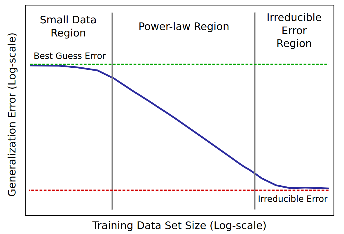
Scaling LLMs
- The more data you train on
- the more the LLM knows about
- the better the LLM generalizes
- scaling law = power law = \(y(x) = ax^{-\gamma} +b\)
- \(y(x) =\) test loss
- \(\gamma\) = slope
Baidu paper 2017
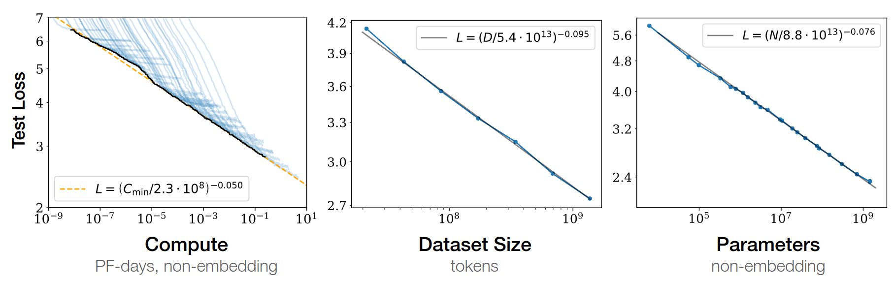
Scaling laws for Neural LM 2020
Open-AI 2020
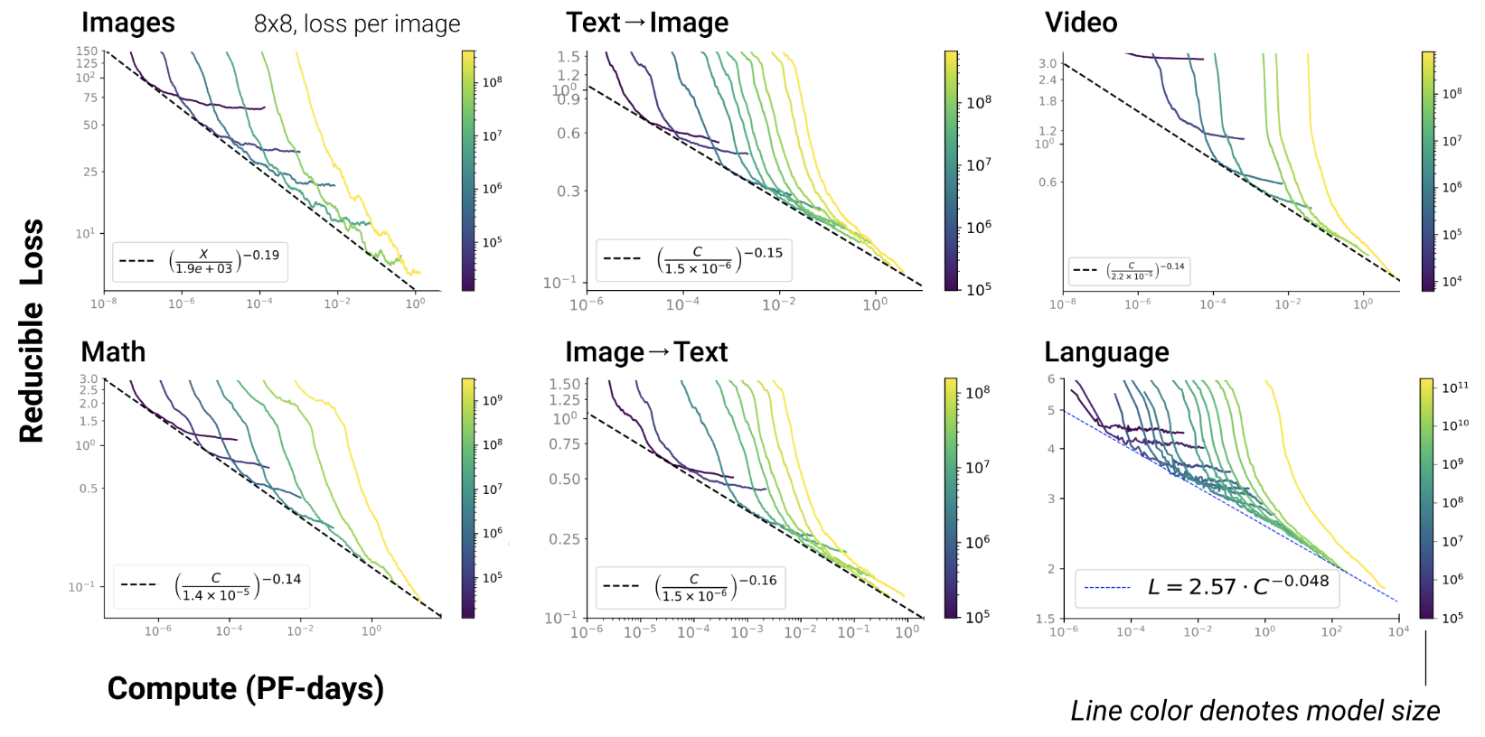
- RL, protein, chemistry…
Chinchilla paper 2022
- GPT3 2020: inc. model capacity
- Chinchilla 2022: inc. data
\(L=\) pretraining loss
Google 2022: paper1, paper2 Flops, Upstream (pretraining), Downstream (acc on 17 tasks), Params
Emerging capabilities
- Scaling laws exist in Machine Learning for a long time (cf. Paper on learning curves)
- But it’s the first time they result from emerging capabilities!
GPT3 paper 2020
- emergence of “In-Context Learning”
- = capacity to generalize the examples in the prompt
- example:
"eat" becomes "ate"
"draw" becomes "drew"
"vote" becomes
Anthropic paper 2022
- shows that the scaling law results from combination of emerging capabilities
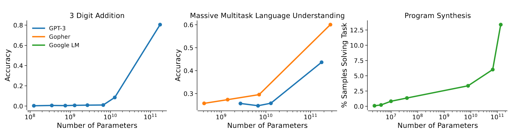
Jason Wei has exhibited 137 emerging capabilities:
- In-Context Learning, Chain-of-thought prompting
- PoT, AoT, Analogical prompting
- procedural instructions, anagrams
- modular arithmetics, simple maths problems
- logical deduction, analytical deduction
- physical intuition, theory of mind ?
- …
Phase transitions during training
During training, LLMs may abruptly reorganize their latent representation space
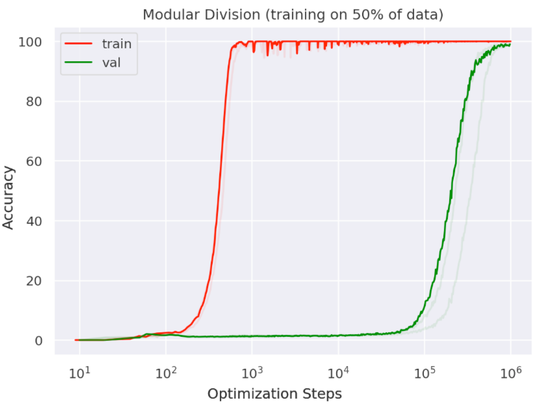
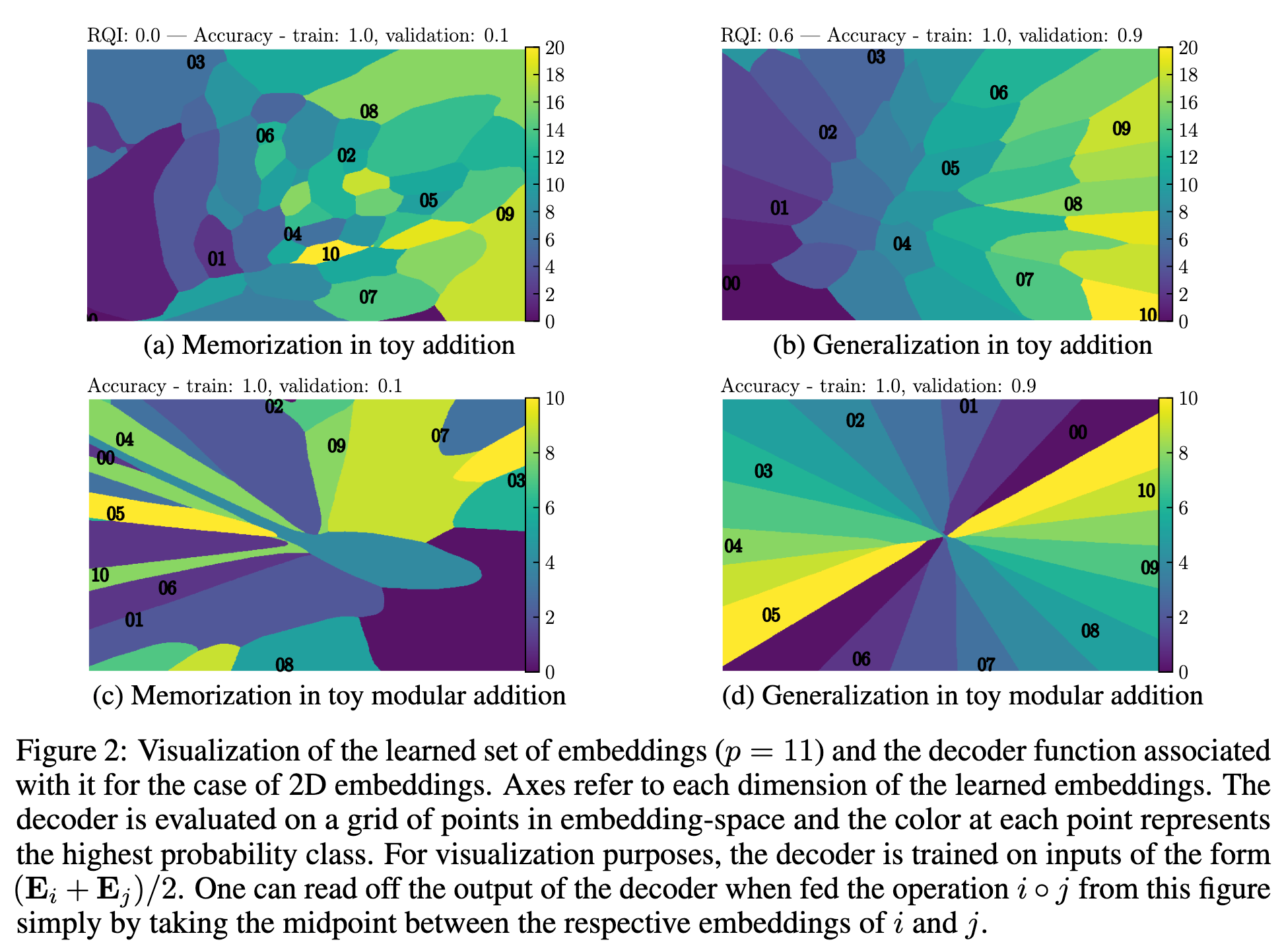
Grokking exhibits structured latent space
LLM traning dynamics
- High-dim training is not a “continuous”/regular process:
- Phase transitions first observed in 2015 in ConvNets
- Later studied in LLMs
- Traditional ML precepts invalidated:
- Overfitting is not bad
- Finding global optimum is not required
Definitions
- Loss = LLM error function to be minimized during training
- Loss landscape = surface/manifold of the loss \(L(\theta)\) as a function of LLM parameters \(\theta\)
- SGD = training algorithm that iteratively updates \(\theta\) following the direction of the gradient \(-\nabla_{\theta} L\) to progressively reduce the error \(L(\theta)\) made by the LLM on the training corpus
- Objective of training = finding a good \(\theta^*\) that gives the smallest possible \(L(\theta)\)
- This can be viewed as navigating on the loss landscape to find a minimum/valley in the loss landscape
- Overfitting = “learning by heart” the training dataset
- = finding an optimal \(\theta^*\) that gives a minimum \(L(\theta)\) on the training corpus, but a large loss on another corpus
- The real objective of training is to find a \(\theta^*\) that generalizes, i.e., that has a low error on other datasets than the training corpus
- Regularization = Ways to prevent overfitting and still get generalization
- reduce nb of parameters, minimize \(||\theta||^2\), dropout, reduce batch size, add noise to data…
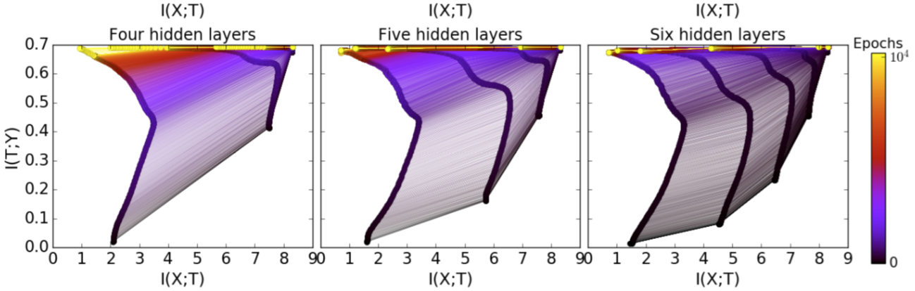
Tishby’s bottleneck
- deep learning creates 2 training phases: overfitting, then compression
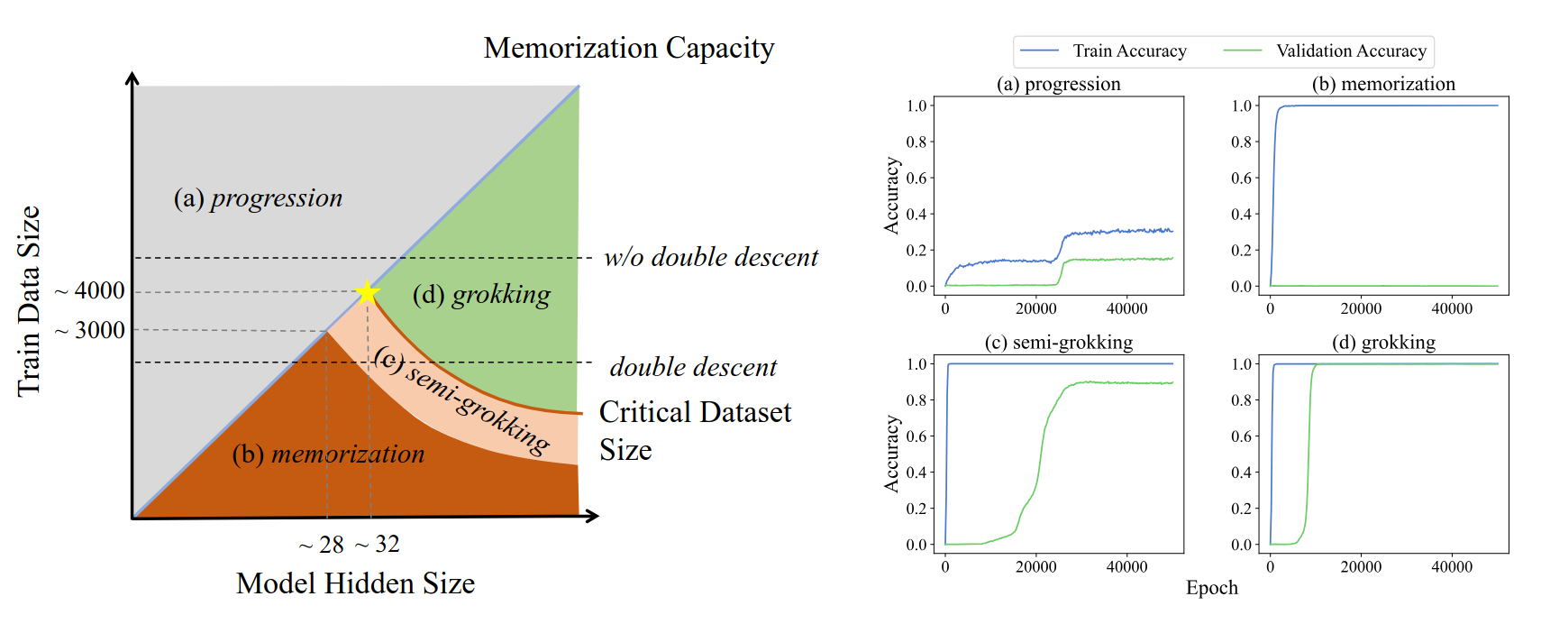
Double descent
First proof that overfitting may be addressed by increasing the nb of parameters!

- Double descent occurs when:
- the model is over-parameterized
- there’s a strong regularization (e.g., L2)
- Intuition:
- With more parameters, many optima exists
- With the help of regularization, the model may find a really good one
Warning
- grokking is a phase transition that occurs during training
- double descent is not a transition of phase that occurs during training!
- double descent helps to understand the necessary conditions for grokking
Back to grokking
- First observed by Google in Jan 2022
- Trained on arithmetic tasks
- Must wait well past the point of overfitting to generalize
- It often occurs “at the onset of Slingshots” Apple paper
- Slingshots = type of weak regularization = when “numerical underflow errors in calculating training losses create anomalous gradients which adaptive gradient optimizers like Adam propagate” blog
- post-grokking solutions = flatter minima
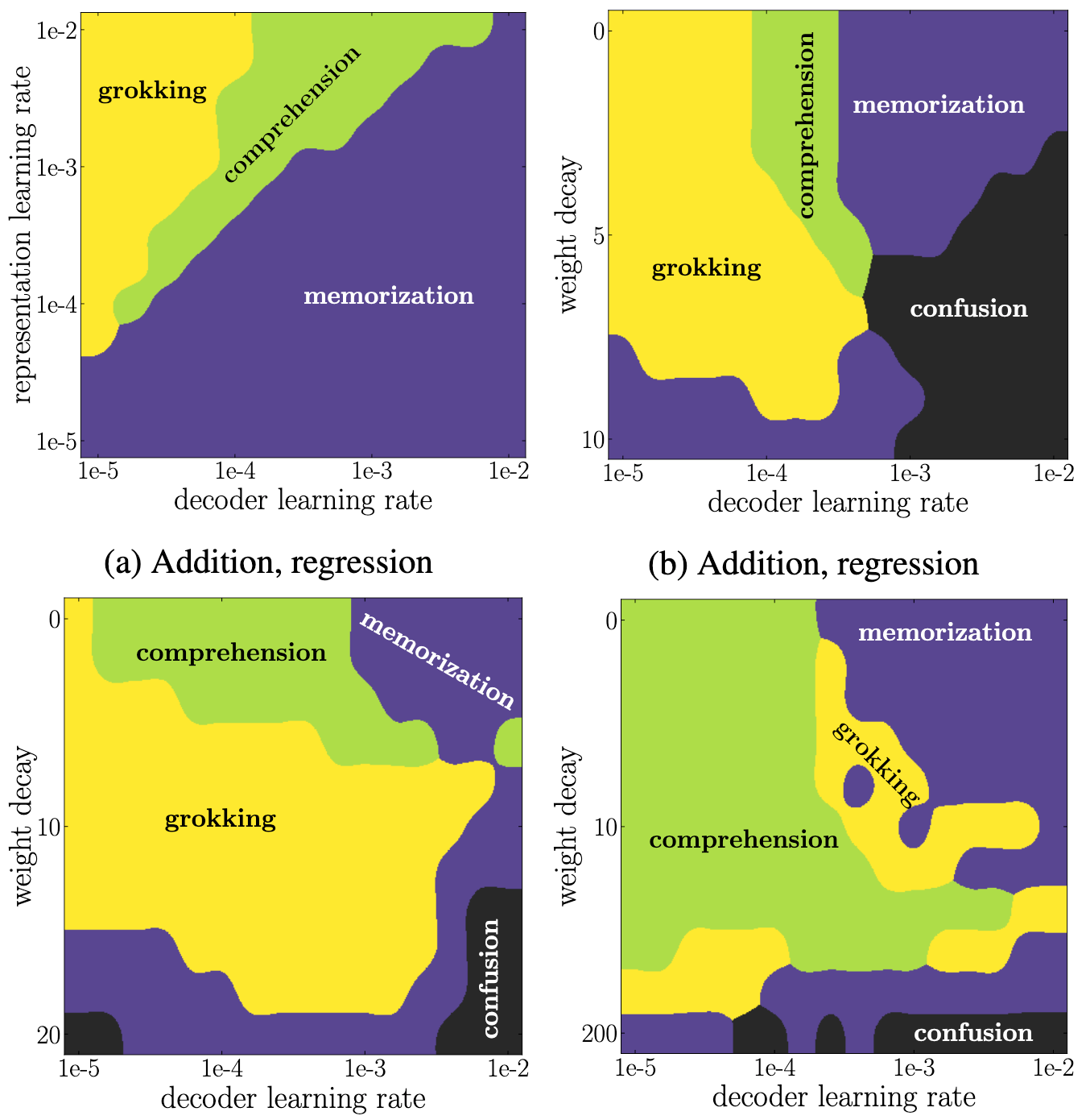
- Training involves multiple phases: grokking is one of them MIT paper
- generalization, grokking, memorization and confusion
- When representations becomes structured, then generalization occurs:
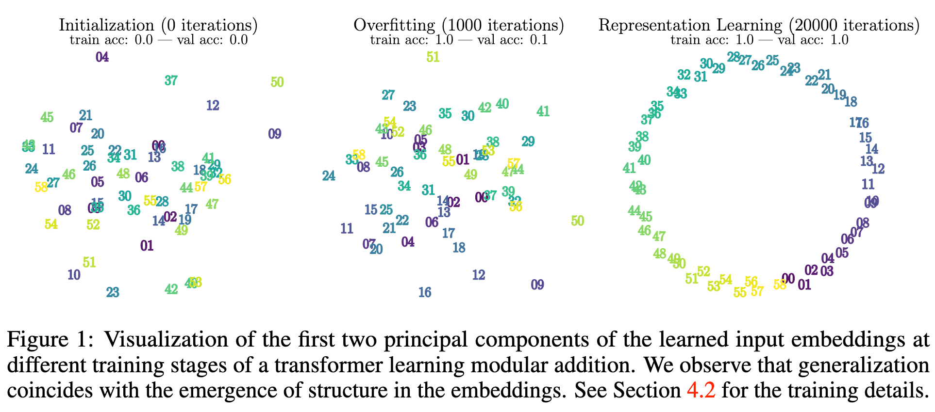
- The 4 phases depend on hyper-parameters:
- Why do we observe phases during training?
- NYU paper 2023
- Because of competing sub-networks: dense for memorization and another sparse for generalization
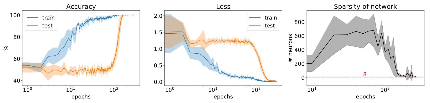
- COLM’24 paper: dual view of double descent and grokking, and training regimes
Wrap-up: scaling parameters
- It’s theoretically better to have over-parameterized models, as it unlocks double descent and potentially grokking
- But Kaplan’s law were promoting too large LLMs, Chinchilla’s law make it more reasonable
- Scaling laws are precious tools to design experiments before starting training
- We know since 2015 that training deep models involve multiple phases
- We now know that LLMs have 4 possible phases, depending on the hyper-parameters
- We know these phase transitions come from competing sub-networks (impossible without over-parameterization)
Case study: Llama3.1
- Main constraint = training compute = \(3.8\times 10^{25}\) FLOPs
- Chinchilla scaling laws not precise enough at that scale, and not for end-task accuracy
- so they recompute they own scaling laws on ARC challenge benchmark!
- They fix compute \(c\) (from \(10^{18}\) to \(10^{22}\) FLOPs)
- They pick a model size \(s\), deduce from \((s,c)\) the nb of data points \(d\) the model can be trained on
- They train it, get the dev loss \(l(s,c,d)\)
- They plot the point \((x=d,y=l)\) and iterate for a few other \(s\)
- For each \(c\), they get a quadratic curve: why?
- Because:
- the largest model is more costly to train, so it’s trained on the fewest data (\(x_{min}\))
- when it’s too large, it’s trained on too few data \(\rightarrow\) high loss
- the smallest model is trained on lots of data (\(x_{max}\))
- but it has too few parameters to memorize information \(\rightarrow\) high loss
- so there’s a best compromise in between
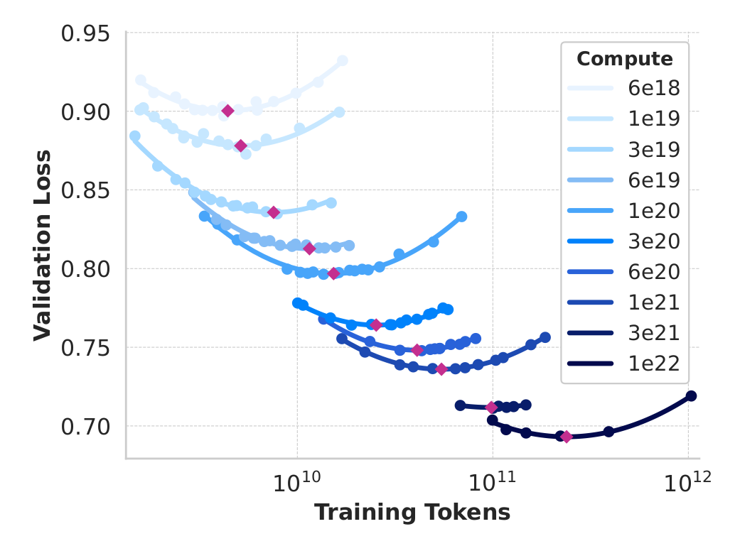
- Terms to remind:
- compute = nb of operations to train
- IsoFLOP curve = plot obtained at a constant compute
- compute-optimal model = minimum of an IsoFLOP curve
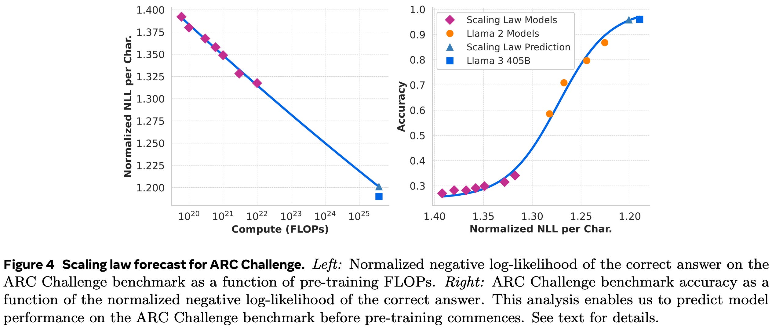
- But these scaling laws are mostly computed at “low” FLOPs range
- So they compute for these models & the largest llama2 models both the dev loss and accuracy
- Assume accuracy = sigmoid(test loss)
- Extrapolate the scaling law with this relation, and get 405b parameters
More and more scaling laws are computed over time, as compute increase, or considering other conditions, architectures:
- Data-constrained scaling laws
- Scaling laws for batch size https://arxiv.org/pdf/2412.01505
- Parallel/ensembling scaling laws paper
- Finetunig scaling laws paper
- Multi-lingual scaling laws: ATLAS (oct 2025)
- …
Design of LLM
Choice of architecture
- Focus on representations: RAG, multimodal, recommendation
- contrastive learning: S-BERT, BGE, E5
- Classification: BERT? More and more: GPT
- Focus on generation:
- Transformer-based (GPT family)
- MoE
- SSM: S4, Mamba
- Diffusion
Mixture of Experts
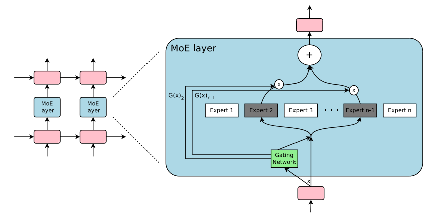
(from huggingface)
Mixture of Experts
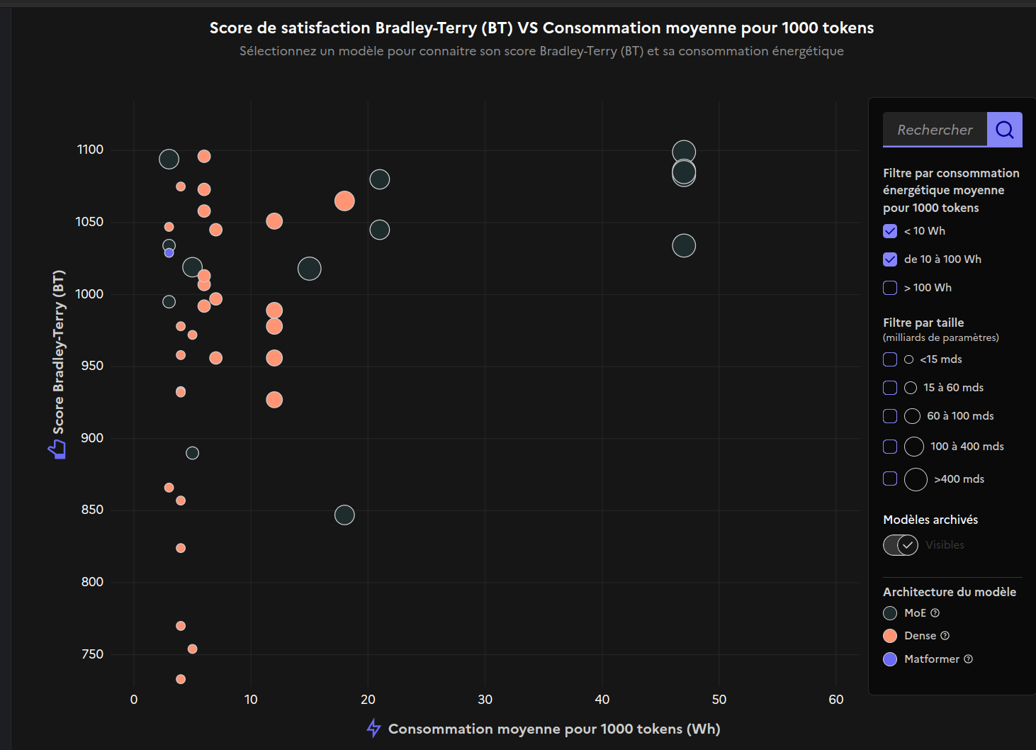
- Main advantage: reduced cost
- Ex: 24GB VRAM (4-bit Mixtral-8x7b) 7b-params during forward pass
- Drawbacks:
- more redundancy across parameters
- hard to train
But MoE may not be that efficient after all… https://comparia.gouv.fr
State-Space Models
- Discrete SSM equation similar to RNN:
\[h_t = Ah_{t-1} + Bx_t\] \[y_t = Ch_t + D x_t\]
- but A,B,C,D are computed: they depend on the context
Mamba
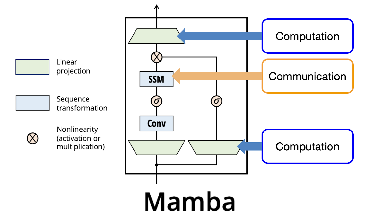
Ex: Mamba
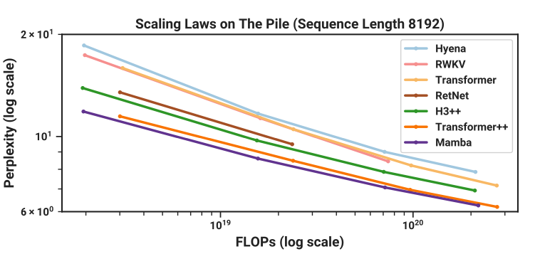
- scaling law comparable to transformer (up to \(10^{20}\) PFLOPs)
- linear \(O(n)\) in context length
- faster inference, but slower training
Diffusion transformer
- Diffusion models: forward noise addition
- Adds noise, step by step to input \[q(x_t|x_{t-1}) = N(x_t;\sqrt{1-\beta_t} x_{t-1}, \beta_t I)\]
- backward denoising process
- starts from white noise
- reverse the forward process with a model (U-Net or transformer): \[p_\theta(x_{t-1}|x_t) = N(x_{t-1}, \mu_\theta(x_t,t), \Sigma_\theta(x_t,t))\]
- iteratively denoise
Many text diffusion models

(from PMC24)
Comparison
- Diffusion models are much slower than LLM, because of many sampling steps
- But they produce a complete sentence at each step
Prompt engineering
- Prompt = input (text) to the LLM
- composed of: system prompt, context, instructions, query, dialogue history, tools…
- A lot can be done without finetuning, just by changing the prompt
- The prompt depends on the model type:
- Foundation model: “text continuation” type of prompt; think as if it’s a web page
- Instruct LLM: add instructions
- Chat LLM: add dialogue history
- Coder LLM: add pieces of code…
- Relies on In-Context Learning capability
- Vanilla prompting
- Chain-of-thought (CoT)
- Self-consistency
- Ensemble refinment
- Automatic chain-of-thought (Auto-CoT)
- Complex CoT
- Program-of-thoughts (PoT)
- Least-to-Most
- Chain-of-Symbols (CoS)
- Structured Chain-of-Thought (SCoT)
- Plan-and-solve (PS)
- MathPrompter
- Contrastive CoT/Contrastive self-consistency
- Federated Same/Different Parameter self-consistency/CoT
- Analogical reasoning
- Synthetic prompting
- Tree-of-toughts (ToT)
- Logical Thoughts (LoT)
- Maieutic Prompting
- Verify-and-edit
- Reason + Act (ReACT)
- Active-Prompt
- Thread-of-thought (ThOT)
- Implicit RAG
- System 2 Attention (S2A)
- Instructed prompting
- Chain-of-Verification (CoVe)
- Chain-of-Knowledge (CoK)
- Chain-of-Code (CoC)
- Program-Aided Language Models (PAL)
- Binder
- Dater
- Chain-of-Table
- Decomposed Prompting (DeComp)
- Three-Hop reasoning (THOR)
- Metacognitive Prompting (MP)
- Chain-of-Event (CoE)
- Basic with Term definitions
- Basic + annotation guideline + error-analysis- lists the best prompting techniques for every possible NLP task.
- Another survey of prompt engineering
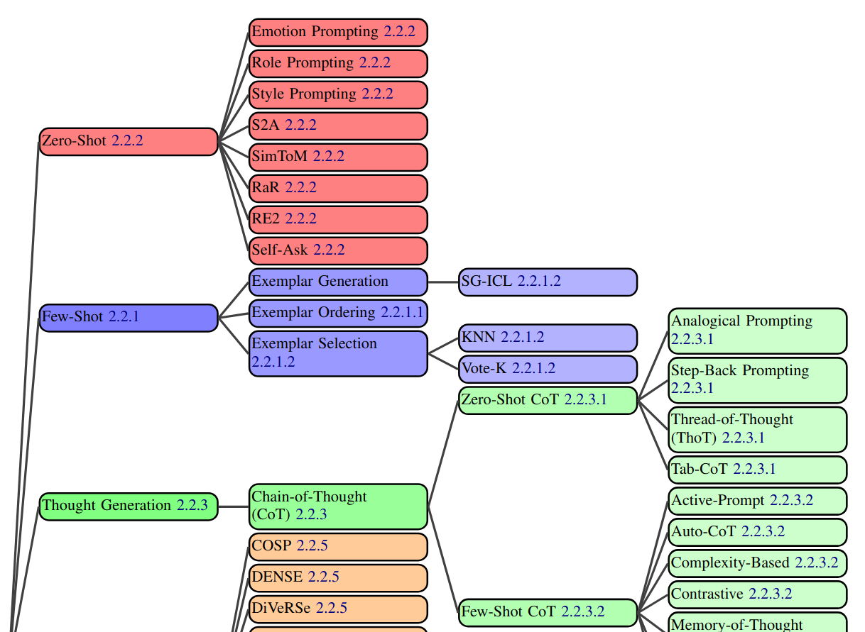
Prompt engineering
- It’s the process/workflow to design a prompt:
- define tasks
- write prompts
- test prompts
- evaluate results
- refine prompts; iterate from step 3
Template of prompt
<OBJECTIVE_AND_PERSONA>
You are a [insert a persona, such as a "math teacher" or "automotive expert"]. Your task is to...
</OBJECTIVE_AND_PERSONA>

<INSTRUCTIONS>
To complete the task, you need to follow these steps:
1.
2.
...
</INSTRUCTIONS>

------------- Optional Components ------------

<CONSTRAINTS>
Dos and don'ts for the following aspects
1. Dos
2. Don'ts
</CONSTRAINTS>

<CONTEXT>
The provided context
</CONTEXT>

<OUTPUT_FORMAT>
The output format must be
1.
2.
...
</OUTPUT_FORMAT>

<FEW_SHOT_EXAMPLES>
Here we provide some examples:
1. Example #1
  Input:
  Thoughts:
  Output:
...
</FEW_SHOT_EXAMPLES>

<RECAP>
Re-emphasize the key aspects of the prompt, especially the constraints, output format, etc.
</RECAP>
Best practices
- Do not start from scratch, better use a template or example of prompt
- the role/persona is important:
- It can be used to generate synthetic data
- To get variable outputs, much better to change the persona than generate with beam search
- may use prefixes for simple prompts:
TASK:
Classify the OBJECTS.

CLASSES:
- Large
- Small
OBJECTS:
- Rhino
- Mouse
- Snail
- Elephant- may use XML or JSON for complex prompts
Few-Shot Learning
- Add a few examples of the task in the prompt
- requires large enough LLM
- few-shot examples are mainly used to define the format, not the content!
Asking for explanations
What is the most likely interpretation of this sentence? Explain your reasoning. The sentence: “The chef seasoned the chicken and put it in the oven because it looked pale.”
Llama3.1-7b: “[…] the chef thought the chicken was undercooked or not yet fully cooked due to its pale appearance […]”
Yes: CoT/explanations may produce a good reasoning/explanation
No: it may be wrong; it does not represent the real reasoning process the LLM used; CoT may not be understandable at all.
CoT workflow
- break the pb into steps
- find good prompt for each step in isolation
- tweak the steps to work well together
- enhance with finetuning:
- generate synthetic samples to tune each step
- finetune small LLMs on these samples
CoT for complex tasks
Extract the main issues and sentiments from the customer feedback on our telecom services.
Focus on comments related to service disruptions, billing issues, and customer support interactions.
Please format the output into a list with each issue/sentiment in a sentence, separated by semicolon.

Input: CUSTOMER_FEEDBACK
Classify the extracted issues into categories such as service reliability, pricing concerns, customer support quality, and others.
Please organize the output into JSON format with each issue as the key, and category as the value.
Input: TASK_1_RESPONSEGenerate detailed recommendations for each category of issues identified from the feedback.
Suggest specific actions to address service reliability, improving customer support, and adjusting pricing models, if necessary.
Please organize the output into a JSON format with each category as the key, and recommendation as the value.
Input: TASK_2_RESPONSECoT for simpler tasks
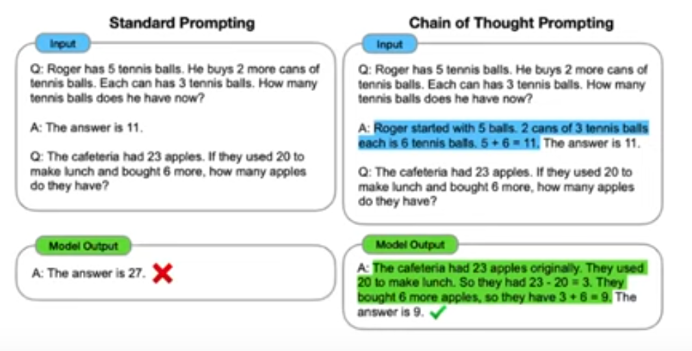
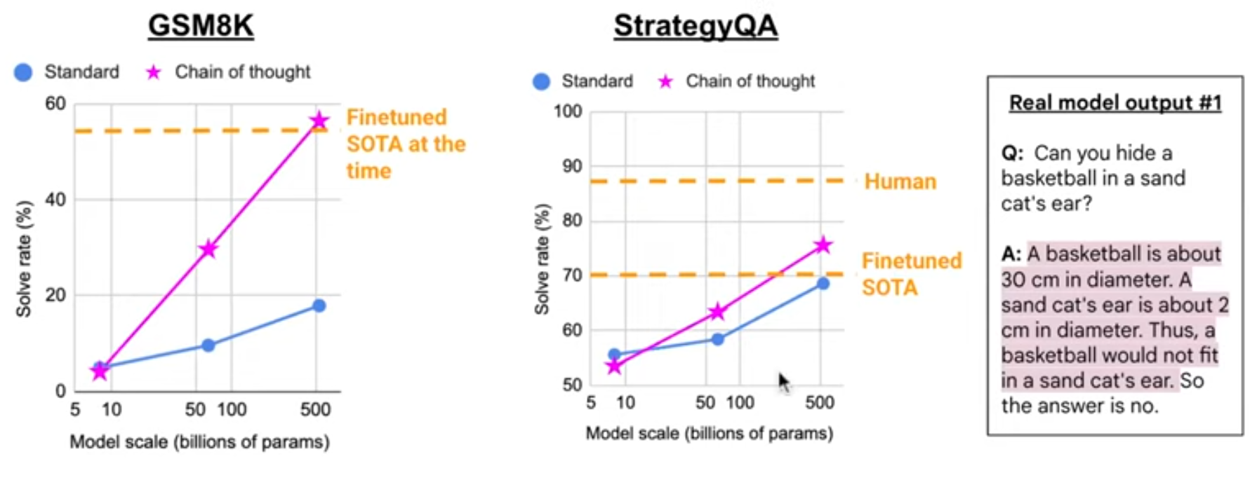
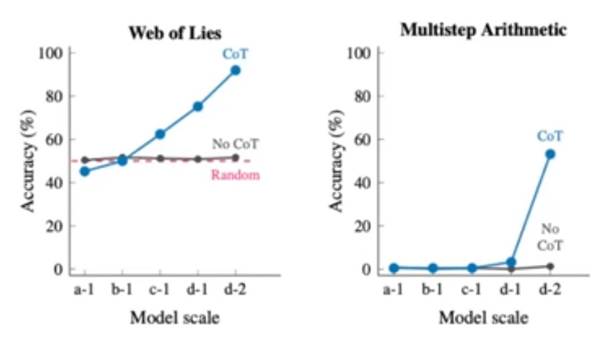
CoT requires large models:
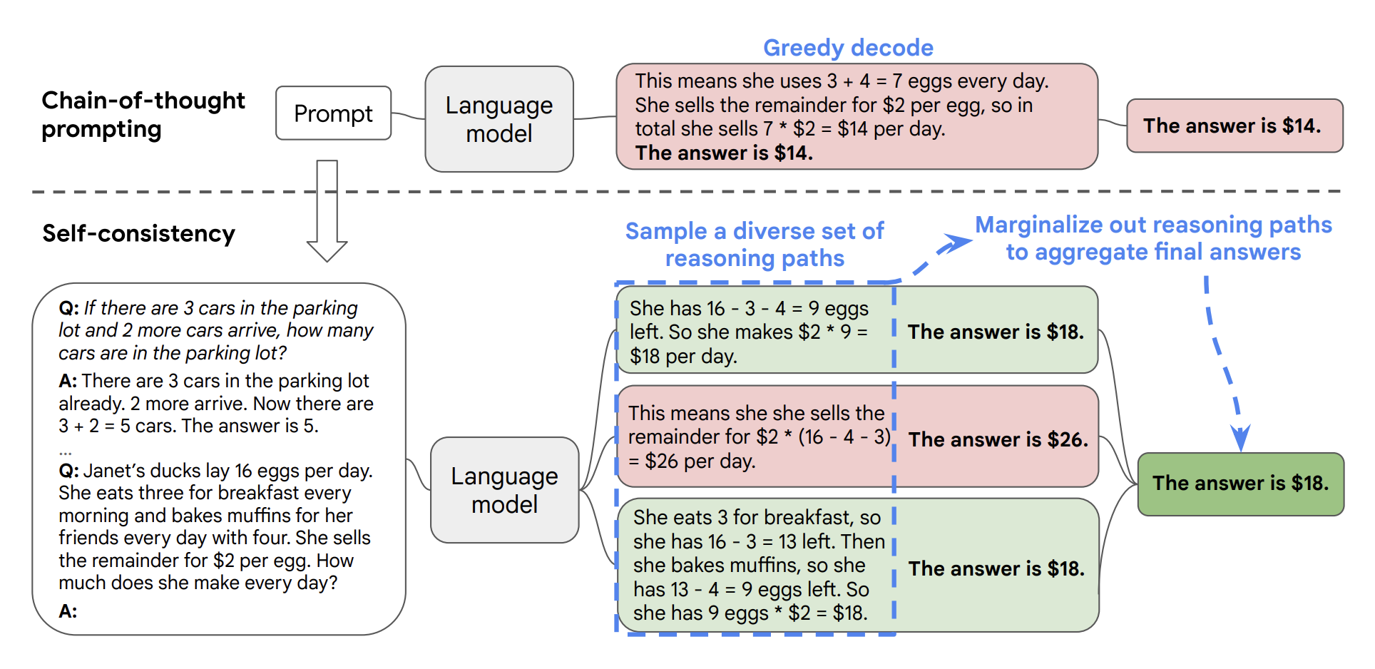
Self-consistency
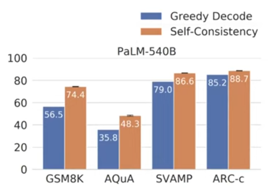
- Self-consistency greatly improves CoT prompting
- For one (CoT prompts, question) input, sample multiple outputs
- take majority vote among outputs
Analogical prompting
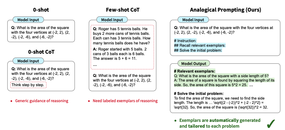
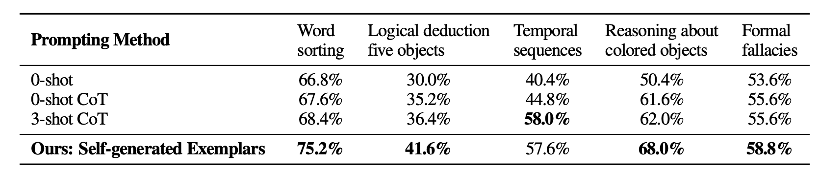
- Few-Shot with self-generated examples:
Algorithm of Thoughts
- Gives a more constrained thinking process than CoT
- Describe the algorithm that the LLM should follow
You are a reasoning agent that must follow an explicit Algorithm of Thoughts.
Do not skip steps. Do not add free-form reasoning.
Follow the algorithm exactly as defined.

Problem
Navigate a 5×5 maze from Start (S) to Goal (G).

Maze representation (row, column):

[
 ["S", ".", "#", ".", "."],
 [".", ".", "#", ".", "#"],
 ["#", ".", ".", ".", "#"],
 ["#", "#", ".", "#", "."],
 [".", ".", ".", ".", "G"]
]

. = open cell
# = wall
Movement allowed: Up, Down, Left, Right
No diagonal moves
Maze indices start at (0,0) in the top-left

Algorithm of Thoughts

State
- Current position (row, column)
- Visited cells set
- Path taken so far (ordered list of moves)

Operators
- Move Up: (r−1, c)
- Move Down: (r+1, c)
- Move Left: (r, c−1)
- Move Right: (r, c+1)

A move is valid if:
- The target cell is inside the grid
- The target cell is not a wall (#)
- The target cell has not been visited

Control Strategy
- Use Breadth-First Search
- Expand states level by level
- Apply operators in this fixed order: Up, Down, Left, Right

Evaluation
A state is successful if the current position equals the goal position

Termination
Stop when the goal is reached
If no states remain, return "No path found"

Execution Rules
At each step, output:
- Current position
- Valid moves generated
- Updated path

Do not explain decisions in natural language
Only follow the defined algorithm

Final Output Format
Path found:
Moves: [Right, Down, Down, ...]
Cells visited: [(0,0), (0,1), ...]

Begin execution.
Tree of Thoughts
- Specific for exploration with backtracking
- Better suited than AoT for maze solving
You are a reasoning agent using Tree of Thoughts.
You must explore multiple candidate reasoning paths in parallel, evaluate them, and prune weak paths.
Do not follow a single linear reasoning chain.

Problem
Navigate a 5×5 maze from Start (S) to Goal (G).

Maze representation (row, column):

[
 ["S", ".", "#", ".", "."],
 [".", ".", "#", ".", "#"],
 ["#", ".", ".", ".", "#"],
 ["#", "#", ".", "#", "."],
 [".", ".", ".", ".", "G"]
]

. = open cell
# = wall
Moves allowed: Up, Down, Left, Right
No diagonal moves
Maze indices start at (0,0) in the top-left

Tree of Thoughts Framework

State
Each thought (node) contains:
- Current position (row, column)
- Visited cells
- Path so far (moves + coordinates)

Thought Expansion
At each state:
- Generate up to 4 candidate next thoughts (one per valid move).
- Each candidate represents a new state after that move.

Evaluation Function
Score each candidate thought from 1 (bad) to 5 (excellent) based on:
- Distance to goal (closer is better)
- No revisiting cells
- Not leading into dead ends

Search Strategy
- Use beam search with width = 2

At each depth:
- Keep only the top 2 highest-scoring thoughts
- Discard all others

Termination Conditions
- If any thought reaches the goal, stop and return the best path
- If all thoughts are dead ends, return "No path found"

Execution Rules
At each depth level:
- List all generated thoughts
- Provide their evaluation scores
- Explicitly state which thoughts are kept and which are pruned
- Do not use natural-language explanations beyond scoring and pruning

Final Output Format

Solution Path:
Moves: [Down, Right, Right, ...]
Cells: [(0,0), (1,0), ...]

Search Tree Summary:
Depth 0: kept thoughts [...]
Depth 1: kept thoughts [...]
...

Begin Tree of Thoughts search.- In the above example, the LLM itself is doing all the job in one call: that’s OK for easy problems, but it often fails
- It’s best to control the search outside the LLM and call the LLM to generate solutions and evaluate them
Ex: Game of 24. First prompt:
Input: 4, 6, 8, 10
Possible next steps:
4+6 = 10 (left: 10, 8, 10)
8-4 = 4 (left 4, 6, 10)
10+4 = 14 (left: 14, 6, 8)

Input: 4 9 10 13
Possible next steps:
Second prompt:
Evaluate if the numbers can reach 24 ( sure/likely/impossible)
10 14: 10+14 = 24 sure
10 7 2: 7*2+10 = 24 sure
11 11: 11 + 11 = 22 impossible
13, 10, 13:
Third prompt:
Input: 4, 6, 8, 10
Possible next steps:
4+6 = 10 (left: 10, 8, 10)
8-4 = 4 (left 4, 6, 10)
10+4 = 14 (left: 14, 6, 8)

Input: 4 9 10 13
Possible next steps:
And so on…
- Game of 24:
- CoT accuracy = 4%
- ToT accuracy = 74%
- ToT helps with puzzles, crosswords, and similar reasoning tasks
ToT for creative writing:
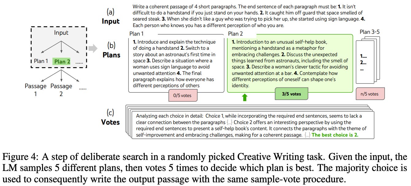
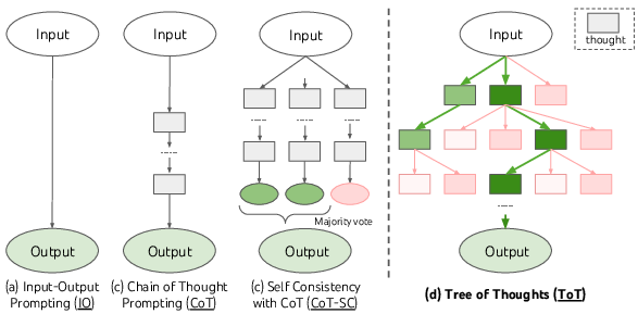
Tool usage
- Also known as “function calling”
- Requirement at the basis of “LLM agents”
There are things an LLM can’t do, so let’s make it call external tools!
LLM agents
- LLM agents = one or multiple LLMs collaborating together and with external tools
- relies on function calling, planner/reasoner, code writer (see Dynasaur)
- Acknowledge that LLM cannot do everything well, so delegate specific tasks to dedicated tools:
- web search, calculator, logic reasoner…
- Often also requires planning:
- An LLM decomposes a complex problem into subtasks (= plan)
- It then assigns the subtasks to other LLMs
- It collect their outputs and iterate or give the final answer
How can an LLM use a tool?
Principle:
- describe in the prompt the tools it can use
- specifiy in the prompt that it can call these tools when he needs to
- parse the LLM’s output for such call requests
- execute externally these calls
- call again the LLM copying the tools’ results in the prompt
Important note:
- Not all LLMs are good at calling tools!
- We need to finetune them to do it well
- Examples:
- Cohere CommandR+ (one of the first tool-specialized LLM)
- LLama-3.1-7b can call tools, but it’s not good at conversation mode with tools
- Llama-3.1-70b handles conversations fine
- Qwen-2.5 are good at tools
- Most post-Llama-3.1 LLMs include tools usage
- Because LLMs are finetuned on function calling, you must use the same format to describe tools
- Typical format used = ChatML, JSON
- Most LLM-wrapper software propose/support a standard way to call tools (see below)
- Note: there’re also specific ways to handle conversation mode, inserting code, adding image, etc.
Chat template
- Raw inputs to LLM are expressed in a structured text format that follows a chat template
- High-level libraries a JSON format (called “OpenAI Chat Completion API”)
{
  "model": "gpt-3.5-turbo",
  "messages": [
    {"role": "system", "content": "Tu est un assistant utile."},
    {"role": "user", "content": "Bonjour !"}
  ]
}- ChatML (Chat Markup Language): GPT-3.5, GPT-4, Qwen2.5, Yi…
<|im_start|>system
You are a helpful assistant.<|im_end|>
<|im_start|>user
Hello!<|im_end|>
<|im_start|>assistant
Hi! How can I help you today?<|im_end|>
<|im_start|>user
What's the weather?<|im_start|>assistant- Llama 3.2…:
<|begin_of_text|><|start_header_id|>system<|end_header_id|>

Tu es un assistant.<|eot_id|><|start_header_id|>user<|end_header_id|>

Bonjour !<|eot_id|><|start_header_id|>assistant<|end_header_id|>
- Mistral, Mixtral…:
<s>[INST] You are a helpful assistant. [/INST]
Hi! How can I help you today?</s>
[INST] Hello! [/INST]- Gemma…:
<start_of_turn>user
Bonjour !<end_of_turn>
<start_of_turn>assistant- Old formats, as Vicuna/Alpaca…:
USER: Bonjour !
ASSISTANT:- The model file (eg. gguf) contains the chat template in Jinja format
- ex for chatMLP:
{% for message in messages %} {{ '<|im_start|>' + message['role'] + '\n' + message['content'] + '<|im_end|>\n' }} {% endfor %} {% if add_generation_prompt %} {{ '<|im_start|>assistant\n' }} {% endif %} - llama.cpp renders the jinja file with its Minja interpreter
- Huggingface models store chat template in file tokenizer_config.json
How to use it with Transformers (see HF course):
from transformers import AutoTokenizer

tokenizer = AutoTokenizer.from_pretrained("Qwen/Qwen3-0.6B")
messages = [
    {"role": "user", "content": "What is 42?"}
]
text = tokenizer.apply_chat_template(
    messages,
    tokenize=False,
    add_generation_prompt=True,
    enable_thinking=True
)
print(text)
JSON for multimodal inputs:
messages = [
    {
        "role": "system",
        "content": "You are a helpful vision assistant that can analyze images.",
    },
    {
        "role": "user",
        "content": [
            {"type": "text", "text": "What's in this image?"},
            {"type": "image", "image_url": "https://example.com/image.jpg"},
        ],
    },
]
For tools use:
messages = [
    {
        "role": "system",
        "content": "You are an AI assistant that can use tools. Available tools: calculator, weather_api",
    },
    {"role": "user", "content": "What's 123 * 456 and is it raining in Paris?"},
    {
        "role": "assistant",
        "content": "Let me help you with that.",
        "tool_calls": [
            {
                "tool": "calculator",
                "parameters": {"operation": "multiply", "x": 123, "y": 456},
            },
            {"tool": "weather_api", "parameters": {"city": "Paris", "country": "France"}},
        ],
    },
    {"role": "tool", "tool_name": "calculator", "content": "56088"},
    {
        "role": "tool",
        "tool_name": "weather_api",
        "content": "{'condition': 'rain', 'temperature': 15}",
    },
]- It’s best to use a ready-to-user software (e.g., HF transformer, ollama…)
- llama-server: expects a JSON-formatted conversation
- llama-cli -cnv: assumes input text = value of “user” key in JSON, then it converts
- llama-cli -p: assumes raw text = you’re responsible!
- If you call yourself the LLM in pytorch, then you have to be very careful about each LLM’s specific tokens, format…
- You can use base LLMs without any chat template; you should use a chat template with instruction tuned LLMs
ReAct prompting
- Principle: Ask the LLM to interleave multiple steps of reasoning and actions
- Workflow:
- First devise few-shot examples
- Adapt a SOTA ReAct prompt
- Test, evaluation, iterate
- ReAct prompt decomposition:
- Primary instruction: “Solve a question answering task…”
- ReAct steps: “… with interleaving Thought, Action, Observation steps”
- Reasoning: “Thought can reason about the current situation”
- Actions: “Actions can be of three types: Search[entity], which searches…; Lookup[keyword], which returns the next sentence containing keyword in the current passage; Finish[answer], which returns the answer and finished the task”
- ReAct few-shot examples:
Question What is the elevation range for the area that the eastern sector of the
Colorado orogeny extends into?
Thought 1 I need to search Colorado orogeny, find the area that the eastern sector
of the Colorado orogeny extends into, then find the elevation range of the
area.
Action 1 Search[Colorado orogeny]
Observation 1 The Colorado orogeny was an episode of mountain building (an orogeny) in
Colorado and surrounding areas.
Thought 2 It does not mention the eastern sector. So I need to look up eastern
sector.
Action 2 Lookup[eastern sector]
Observation 2 (Result 1 / 1) The eastern sector extends into the High Plains and is called
the Central Plains orogeny.
Thought 3 The eastern sector of Colorado orogeny extends into the High Plains. So I
need to search High Plains and find its elevation range.
Aside from the Apple Remote, what other devices can control the program Apple Remote was originally designed to interact with?
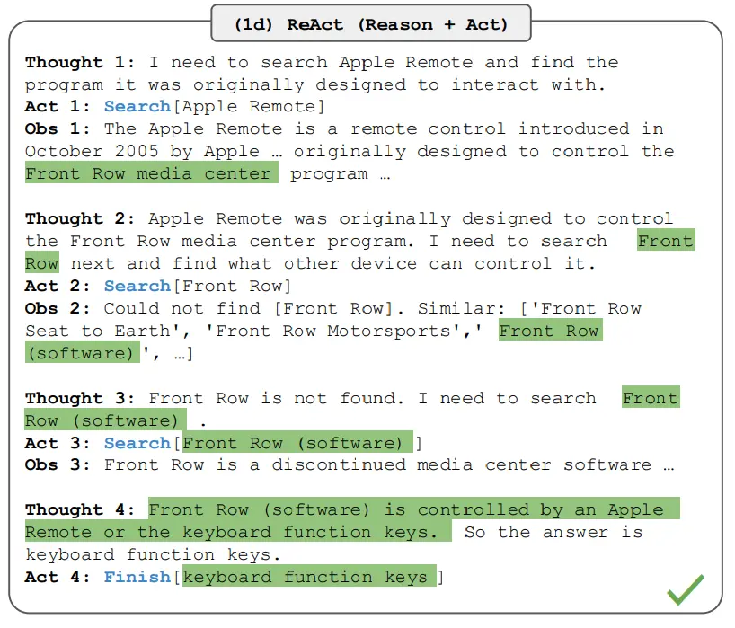
Model Context Protocol
- MCP = standard to connect LLM apps with external apps:
- data and file systems: PostgreSQL, QSLite, GDrive…
- dev tools: git, python executor…
- productivity tools: slack, Google Maps…
- Libs permettent d’intégrer MCP avec ollama, OpenAI, deepseek…: ex: DolphinMCP
Agent best practices
- Agents.md (or gemini.md…):
- central file to provide context + instructions to LLM agents
- README.md are for humans, Agents.md for LLMs.
# Sample AGENTS.md file

## Dev environment tips
- Run `pnpm install --filter <project_name>` to add the package to your workspace so Vite, ESLint, and TypeScript can see it.
- Check the name field inside each package's package.json to confirm the right name—skip the top-level one.

## Testing instructions
- Find the CI plan in the .github/workflows folder.
- Run `pnpm turbo run test --filter <project_name>` to run every check defined for that package.
- From the package root you can just call `pnpm test`. The commit should pass all tests before you merge.
- Fix any test or type errors until the whole suite is green.- First call: make the LLM generate a single markdown file with a plan:
- Summary of the objectives, of the plan
- list of TODOs
- [x] Research visa requirements for Singapore passport holders visiting Japan
- [ ] Compare flight options from Singapore to Tokyo
- [ ] Book flights and hotels once itinerary is finalized- After every action, ask the LLM to
- Update the TODO list
- Update a summary of what has been done
- Read/Write markdown files are the #1 tool for agents:
- They increase long-term planning coherence
- They provide a global, consistent, up-to-date context
- When you design a website, add /robots.txt and /llms.txt
Rise of “AI Environments”
- claude-code, gemini-cli; qwen-code, goose…
- all based on the same principle:
- set of tools (plugins)
- markdown files for constitution, memory, plans, preferences, TODO list…
- connect to “coder LLMs” via API
- abstract control loop: user input, analyse, plan, write, update…
Prompt tuning: DSPy
- DSPy uses LM-driven optimizers to tune prompts and weights
- DSPy concepts:
- LLMs are blackboxes with inputs/outputs described in English
- program = LLMs connected together/used by a program
- compiler = try to find the best prompts
DSPy compilers
- LabeledFewShot: sample randomly examples from training set and add them as demos (few-shots) in the prompt
- BootstrapFewShot:
- create Teacher program = run LabeledFewShot on the Student program
- Evaluate teacher on the train set, keeping when it’s correct
- Add the kept demos as few-shot
- …
Basic usage of DSPy
- launch an LLM provider, e.g., ollama
import dspy
lm = dspy.LM(model="ollama/qwen2.5", api_base="http://localhost:11434")
dspy.configure(lm=lm)
qa = dspy.Predict('question: str -> response: str')
response = qa(question="what are high memory and low memory on linux?")
print(response.response)
dspy.inspect_history(n=1)- What is a typical prompt used for Chain of Thought?
cot = dspy.ChainOfThought('question -> response')
res = cot(question="should curly braces appear on their own line?")
print(res.response)
dspy.inspect_history(n=1)- Let’s evaluate on a MATH benchmark:
from dspy.datasets import MATH

dataset = MATH(subset='algebra')
dev = dataset.dev[0:10]
example = dataset.train[0]
print("Question:", example.question)
print("Answer:", example.answer)

module = dspy.ChainOfThought("question -> answer")
print(module(question=example.question))

evaluate = dspy.Evaluate(devset=dev, metric=dataset.metric)
evaluate(module)- Going further:
Practical session: RAG optimization
- Prompt engineering = manual prompt optimization
- Auto-prompt optimization: DSPy, AdalFlow…
- Components that can be optimized:
- System prompt (CoT)
- Few-shot examples
- LLM parameters…
Implementing a RAG with DSPy; required imports:
import dspy
from dspy.teleprompt import BootstrapFewShot
from dspy.datasets import HotPotQA
from dspy.evaluate import Evaluate
from sentence_transformers import SentenceTransformer
import pandas as pd
from dspy.evaluate.evaluate import Evaluate- Get database of biological documents:
passages0 = pd.read_parquet("hf://datasets/rag-datasets/rag-mini-bioasq/data/passages.parquet/part.0.parquet")
test = pd.read_parquet("hf://datasets/rag-datasets/rag-mini-bioasq/data/test.parquet/part.0.parquet")
passages = passages0[0:20]- Build a retriever on these passages:
class RetrievalModel(dspy.Retrieve):
    def __init__(self, passages):
        self.passages = passages
        self.passages["valid"] = self.passages.passage.apply(lambda x: len(x.split(' ')) > 20)
        self.passages = self.passages[self.passages.valid]
        self.passages = self.passages.reset_index()
        for i,x in enumerate(self.passages.passage.tolist()):
            print("DOC",i,x)
        self.model = SentenceTransformer("all-MiniLM-L6-v2")
        self.passage_embeddings = self.model.encode(self.passages.passage.tolist())

    def __call__(self, query, k):
        query_embedding = self.model.encode(query)
        similarities = self.model.similarity(query_embedding, self.passage_embeddings).numpy() # cosine similarities
        top_indices = similarities[0, :].argsort()[::-1][:k] # pick TopK documents having highest cosine similarity
        response = self.passages.loc[list(top_indices)]
        response = response.passage.tolist()
        return [dspy.Prediction(long_text= psg)  for psg in response]

rm = RetrievalModel(passages)- Test retriever:
qq = "Which cell may suffer from anemia?"
print(rm(qq,2))- Add the generator LLM:
llm = dspy.LM(model="ollama/qwen2.5:0.5b", api_base="http://localhost:11434")
print("llm ok")
dspy.settings.configure(lm=llm,rm=rm)- Define the RAG module:
class GenerateAnswer(dspy.Signature):
    """Answer questions with short factoid answers."""
    context = dspy.InputField(desc="may contain relevant facts")
    question = dspy.InputField()
    answer = dspy.OutputField(desc="often between 1 and 5 words")

class RAG(dspy.Module):
    def __init__(self, num_passages=2):
        super().__init__()
        self.retrieve = dspy.Retrieve(k=num_passages)
        self.generate_answer = dspy.ChainOfThought(GenerateAnswer)
    def forward(self, question):
        context = self.retrieve(question).passages
        prediction = self.generate_answer(context=context, question=question)
return dspy.Prediction(context=context, answer=prediction.answer)- Test your RAG:
rag = RAG()
pred = rag(qq)
print(f"Question: {qq}")
print(f"Predicted Answer: {pred.answer}")
print(f"Retrieved Contexts (truncated): {[c[:200] + '...' for c in pred.context]}")
llm.inspect_history(n=1)- Build a train and dev set:
dataset = []
for index, row in test.iterrows():
    dataset.append(dspy.Example(question=row.question, answer=row.answer).with_inputs("context", "question"))
trainset, devset = dataset[:4], dataset[17:20]- Define an evaluation metric:
def validate_context_and_answer(example, pred, trace=None):
    answer_EM = dspy.evaluate.answer_exact_match(example, pred)
    answer_PM = dspy.evaluate.answer_passage_match(example, pred)
return answer_EM and answer_PM- Evaluate quantitatively your RAG:
valuate_on_devset = Evaluate(devset=devset, num_threads=1, display_progress=True, display_table=10)
evalres = evaluate_on_devset(rag, metric=validate_context_and_answer)
print(f"Evaluation Result: {evalres}")- Add few-shot samples automatically sampled/optimised from the train set:
teleprompter = BootstrapFewShot(metric=validate_context_and_answer, max_bootstrapped_demos=2, max_labeled_demos=2)
compiled_rag = teleprompter.compile(rag, trainset=trainset)
evalres = evaluate_on_devset(compiled_rag, metric=validate_context_and_answer)
print(f"Evaluation Result: {evalres}")
llm.inspect_history(n=1)- TODO:
- run these steps one after the other, and check how the LLM prompt changes
- define a metric that favours short answers and optimize your prompts accordingly
- implement multi-hop RAG in DSPy (see next slides)
- Multi-hop RAG is when decomposing a single RAG query into multiple steps
- The following code shows using a vector-DB
- TODO: in the following code:
- add the LLM with Ollama
- add both missing DSPy signatures
- add more phones from the “Amazon Reviews: Unlocked Mobile Phones” Kaggle dataset
- execute the code
- Multi-hop RAG draft:
import dspy
from dsp.utils import deduplicate
from dspy.teleprompt import BootstrapFewShot
from dspy.retrieve.qdrant_rm import QdrantRM
from qdrant_client import QdrantClient

formatted_list = ["Phone Name: HTC Desire 610 8GB Unlocked GSM 4G LTE Quad-Core Android 4.4 Smartphone - Black (No Warranty)\nReview: The phone is very good , takes very sharp pictures but the screen is not bright'",
        "Phone Name: Apple iPhone 6, Space Gray, 128 GB (Sprint)\nReview: I am very satisfied with the purchase, i got my iPhone 6 on time and even received a screen protectant with a charger. Thank you so much for the iPhone 6, it was worth the wait.",
        ]
client = QdrantClient(":memory:")
def add_documents(client, collection_name, formatted_list, batch_size=10):
    for i in range(0, len(formatted_list), batch_size):
        batch = formatted_list[i:i + batch_size]
        batch_ids = list(range(i + 1, i + 1 + len(batch)))
        client.add(
            collection_name=collection_name,
            documents=batch,
            ids=batch_ids
        )
        print(f"Batch {i // batch_size + 1} added with {len(batch)} documents.")
add_documents(client, "phone_collection", formatted_list)


qdrant_retriever_model = QdrantRM("phone_collection", client)
dspy.settings.configure(lm= llm, rm=qdrant_retriever_model)

class Multihoprag(dspy.Module):
    def __init__(self, passages_per_hop=3, max_hops=2):
        super().__init__()
        self.generate_query = [dspy.ChainOfThought(GenerateSearchQuery) for _ in range(max_hops)]
        self.retrieve = dspy.Retrieve(k=passages_per_hop)
        self.generate_answer = dspy.ChainOfThought(GenerateAnswer)
        self.max_hops = max_hops

    def forward(self, question):
        context = []
        for hop in range(self.max_hops):
            query = self.generate_query[hop](context=context, question=question).query
            passages = self.retrieve(query).passages
            context = deduplicate(context + passages)
        pred = self.generate_answer(context=context, question=question)
        return dspy.Prediction(context=context, answer=pred.answer)

trainset_list = [
  {
    "Question": "Which phones have the best camera quality and battery life based on recent reviews and specifications?",
    "Answer": "Here's a list of phones that meet your criteria:\n\n1. Samsung Galaxy S21 Ultra\n2. Google Pixel 6 Pro\n3. Apple iPhone 13 Pro Max\n4. OnePlus 9 Pro\n5. Xiaomi Mi 11 Ultra\n\nNotes: These phones were picked based on their high ratings for camera quality and long-lasting battery life, as reported by recent reviews and detailed specifications."
  },
  {
    "Question": "What are the top-rated phones with the best display and performance in the market right now?",
    "Answer": "Here's a list of phones that meet your criteria:\n\n1. Samsung Galaxy S22\n2. Apple iPhone 14 Pro\n3. OnePlus 10 Pro\n\nNotes: These phones were selected because they have received excellent reviews for their display clarity and performance speed, making them ideal for users seeking high-quality visuals and efficient processing."
  },
  {
    "Question": "Can you recommend phones that have the best user interface and build quality according to recent user reviews?",
    "Answer": "Here's a list of phones that meet your criteria:\n\n1. Nokia 8.3 5G\n2. Sony Xperia 1 III\n\nNotes: These phones were chosen due to their outstanding user interface design and robust build quality, which have been highly praised in recent user reviews and expert evaluations."
  }
]
trainset = [dspy.Example(question=item["Question"], answer=item["Answer"]).with_inputs('question') for item in trainset_list]

# metric function that prefers short and non-repetitive answers
def validate_answer_and_hops(example, pred, trace=None):
    # if not validate(pred.answer == example.answer): return False
    hops = [example.question] + [outputs.query for *_, outputs in trace if 'query' in outputs]
    if max([len(h) for h in hops]) > 100: return False
    if any(dspy.evaluate.answer_exact_match_str(hops[idx], hops[:idx], frac=0.8) for idx in range(2, len(hops))): return False
    return True

teleprompter = BootstrapFewShot(metric=validate_answer_and_hops, )
uncompiled_rag = Multihoprag()
compiled_rag = teleprompter.compile(student=uncompiled_rag, trainset= trainset)

print(uncompiled_rag("Which smartphones are highly rated for its low-light camera performance also have a great front camera"))

print(compiled_rag("Which smartphones are highly rated for its low-light camera performance also have a great front camera"))
Practical session: ollama
- ollama is designed to be easy to use locally to try out open source LLMs
- it downloads a quantized LLM locally and launch an OpenAI-compatible server
- you can call this server from many available chatGPT-compatible clients
- (Personal note: my preferred client is pure linux command-line: charm.sh mods)
- Ollama also gives simple command-line scripts to immediatly start chatting
- As of 2025, it’s one of the preferred way to quickly start using an LLM.
Q1: Run Qwen-2.5 locally with ollama
- Install ollama locally: follow the instructions at https://ollama.com.
- Check that you can start chatting with Qwen:
ollama pull qwen2.5
ollama run qwen2.5- Note: if you have less than 4GB of RAM, you may want to use a smaller model, like qwen2.5:0.5b, gemma2b, or tinydolphin.
ollama run gemma2:2b- If nothing works, you may run your commands on a free google colab tier.
- Exercice: Ask for a summary of some text file by prepending the string “Summarize this file:” to the actual file content
- Note that the result is very sensitive to the prompt you use: try with various prompts (be creative!) and observe the differences.
{ cat fich.txt; echo "summarize the previous text in 3 lines maximum:"; } | modsQ2: Use Qwen2.5 to interact with tools
- We’re going to call ollama from within python
- Important: When listing the tools/python methods for ollama, it’s important to clearly describe what each method is doing as well as each of its arguments in plain English, as the LLM will decide to call a given tool based on its description!
- Here is a code snippet that shows you how to chat with Qwen2.5 and makes it use a tool
- The tool is a simple function that queries a free website for headline news for a requested country:
import ollama
import requests
import json

messages = [{'role': 'user', 'content': 'What is the main news right now in the USA?'}]

def getnews(c):
    c=c.lower().strip()
    if c=='france': s='fr'
    elif c=='india': s='in'
    elif c=='usa': s='us'
    elif c=='australia': s='au'
    elif c=='russia': s='ru'
    elif c=='united kingdom': s='gb'
    else:
        print("unknown country",c)
        s='fr'
    url="https://saurav.tech/NewsAPI/top-headlines/category/general/"+s+".json"
    print("calling fct")
    response = requests.get(url)
    res = response.text
    print("tool res",res)
    print("\n"*5)

    n=json.loads(res)
    r=n['articles'][0]['title']+": "+n['articles'][0]['content']
    print("extracting news",r,"\n"*3)
    return r

def main():
    response = ollama.chat(
        model='qwen2.5',
        messages=messages,
        tools=[
          {
            'type': 'function',
            'function': {
              'name': 'getnews',
              'description': 'Get recent news from a country',
              'parameters': {
                'type': 'object',
                'properties': {
                    'country': {
                        'type': 'string',
                        'description': 'The name of the country',
                        },
                },
                'required': ['country'],
              },
            },
          },
        ],
    )

    # Add the model's response to the conversation history
    messages.append(response['message'])
    print("first answer",response['message'])

    # Check if the model decided to use the provided function
    if not response['message'].get('tool_calls'):
        print("The model didn't use the function. Its response was:")
        print(response['message']['content'])
        return

    # Process function calls made by the model
    if response['message'].get('tool_calls'):
        available_functions = {
          'getnews': getnews,
        }
        for tool in response['message']['tool_calls']:
          function_to_call = available_functions[tool['function']['name']]
          function_response = function_to_call(tool['function']['arguments']['country'])
          # Add function response to the conversation
          messages.append(
            {
              'role': 'tool',
              'content': function_response,
            }
          )

    # Second API call: Get final response from the model
    final_response = ollama.chat(model='qwen2.5', messages=messages)
    print(final_response['message']['content'])

main()

# adapted from https://github.com/ollama/ollama-python/blob/main/examples/tools/main.py- Test this code, requesting top news from several countries, and ensure that the LLM does indeed make a call to the news scrapper and does not hallucinate fake news.
- Add another for the current weather: I recommend https://wttr.in
- Modify the code so that multiple news, instead of the first news only, are passed to the LLM.
Q3: R/W files
- make a tool to read/write a file in python
- extend to multiple files/dirs
- Then, try with the easy CLI tool orla, which integrates with ollama
Analyzing LLM Training
- Tools to analyze training curves:
- Tensorboard
- Weights And Biases (wandb)
- print() then gnuplot
Tensorboard
- Assuming log files have been generated with the tensorboard format, the tool does:
- Extract the training curves from log files
- Open a web server to visualize them
- Most training libraries create by default tensorboard-compliant logs:
- pytorch lightning
- ms-swift
- …
Logging for tensorboard
- The following code shows how to directly create a log for tensorboard
- copy-paste it and observe the curve
import torch
from transformers import AutoTokenizer, AutoModelForSequenceClassification
import random
from torch.utils.tensorboard import SummaryWriter

writer = SummaryWriter()
tokenizer = AutoTokenizer.from_pretrained('distilbert-base-uncased')
print(tokenizer.special_tokens_map)

class Traindata(torch.utils.data.Dataset):
    def __init__(self):
        super().__init__()
        d = ['a','b']
        self.y = [0,1]
        self.x = tokenizer.batch_encode_plus(d,return_tensors='pt')['input_ids'].split(1)
        print("tokenization done",len(self.x))

    def __len__(self):
        return len(self.x)

    def __getitem__(self,i):
        return self.x[i], self.y[i]


model = AutoModelForSequenceClassification.from_pretrained('distilbert-base-uncased')
for n,p in model.named_parameters():
    if not '.layer.5' in n: p.requires_grad=False
    print(n,p.shape)
opt = torch.optim.SGD(model.parameters(), lr = 1e+5)

traindata = Traindata()
trainloader = torch.utils.data.DataLoader(traindata, batch_size=1, shuffle=True)

for ep in range(100):
    totl = 0.
    for x,y in trainloader:
        opt.zero_grad()
        x = x.view(1,-1)
        yy = torch.LongTensor(y)
        pred = model(x)
        loss = torch.nn.functional.cross_entropy(pred['logits'],yy)
        totl += loss.item()
        loss.backward()
        opt.step()
    print(ep,totl)
    writer.add_scalar("trainloss", totl, ep)

writer.flush()

exit()

# to view the curves:
# tensorboard --logdir=runs/
Analyzing training curves
- It’s the main way to debug your training
- Traditional CS debugging:
- re-read the code (pair reading)
- run an example through the code manually
- …
- Debugging standard code =
- Collecting evidence
- Make hypothesis about what may go wrong
- Check your hypothesis
- Iterate until your hypothesis is correct
- Debugging LLM training =
- Same process \(\rightarrow\) low-level errors
- But LLMs are also “abstract beasts” that may fail in many other ways!
- With LLMs, CS has evolved from an applied math science to an experimental science (like biology, physics, cognitive)
- We can only observe the LLM and try to guess how it works
- We collect evidence, and try to build embryos of theories out of them
- Why do we collect evidence at test time?
- to measure the capabilities of the LLM (e.g. theory of mind)
- to build theories of how it works
- to improve how we can better use it (prompt engineering)
- Why do we collect evidence at training time?
- to detect any of the many ways in which training can fail
- to progressively build trust on our trained model
- when we have the feeling to really understand every evidence we observe, then we can trust our model and deliver it
- What evidence can we observe?
- At inference time:
- input/output pairs
- output logits/probas
- latent representations
- At training time:
- training loss
- validation loss
- learning rate dynamics
- per model, per layer, per matrix:
- gradient norm + dynamics
- parameter norm/peaks + dynamics
- parm updates + dynamics
- matrices rank, mutual info between X/Z and Z/Y…
training and validation losses
- The most important evidence
- Must always be plotted
- Look for their shape, their instabilities, their difference
- Focus on every detail that you do not understand \(\rightarrow\) debug it: make hypothesis to explain it, test your hypothesis, iterate
Training curves zoo
- Next are “typical” training and validatioon curves shapes you should be able to understand
Curve 1
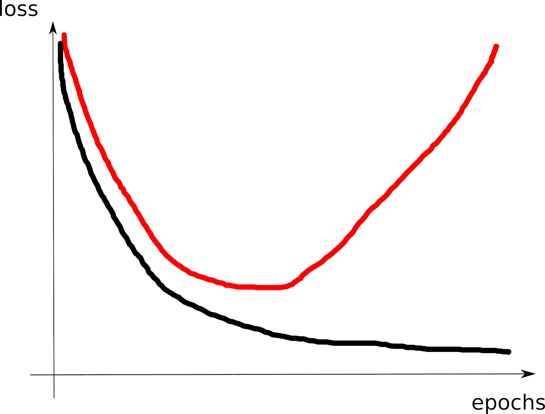
Curve 2
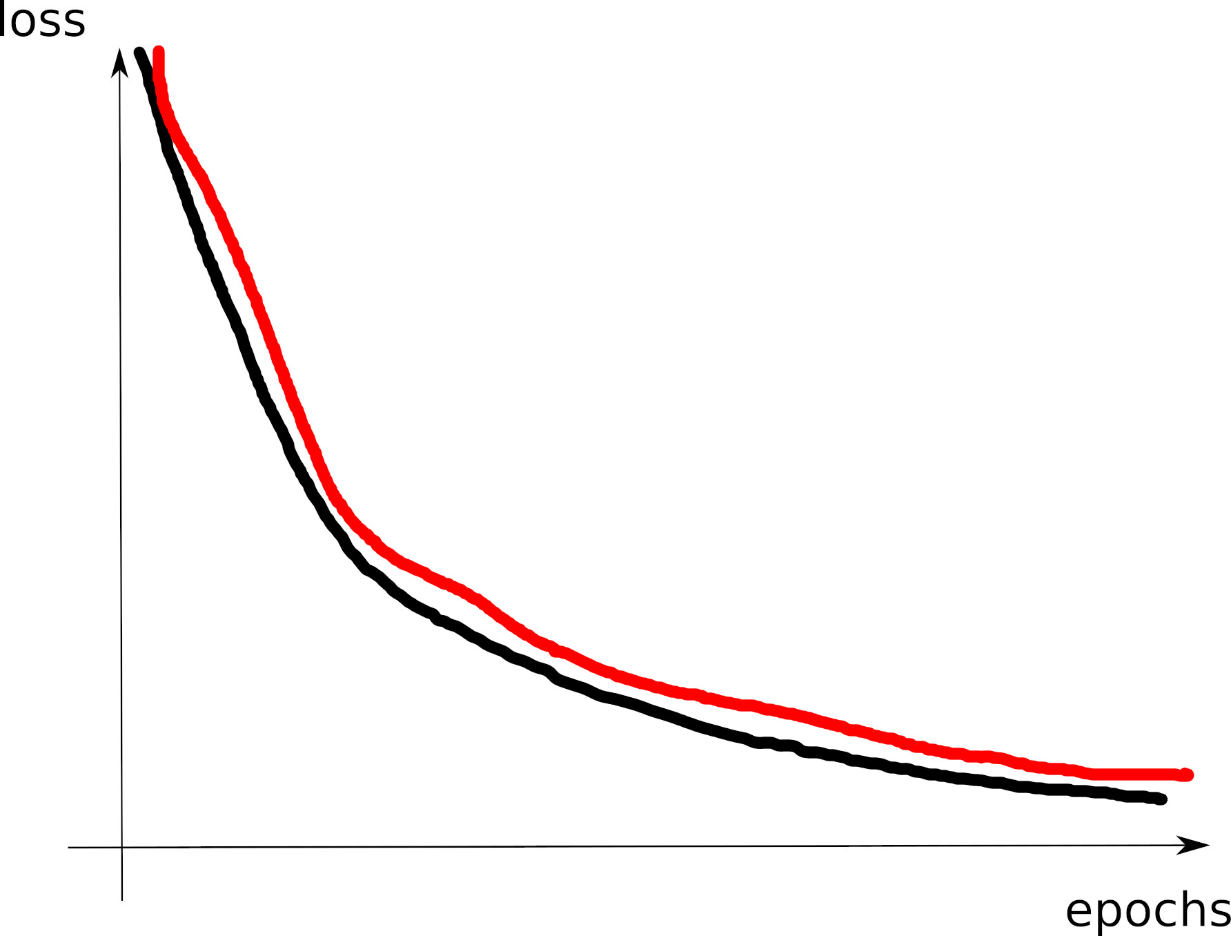
Curve 3
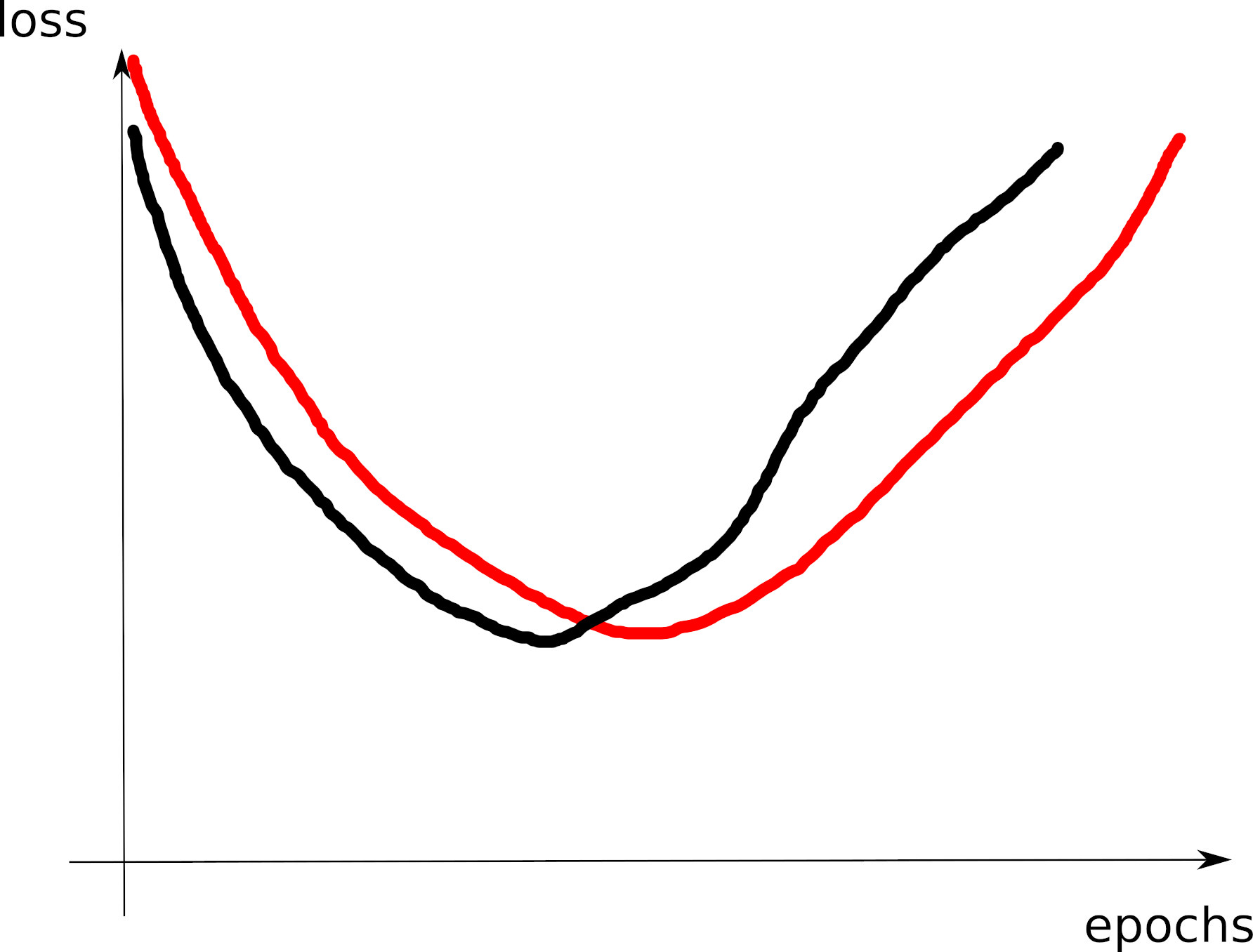
Curve 4
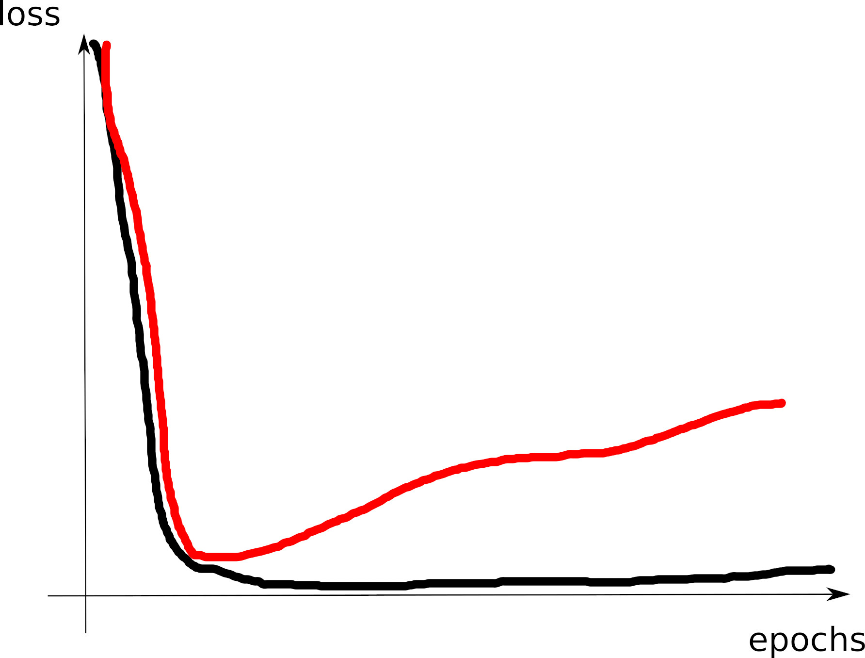
Curve 5
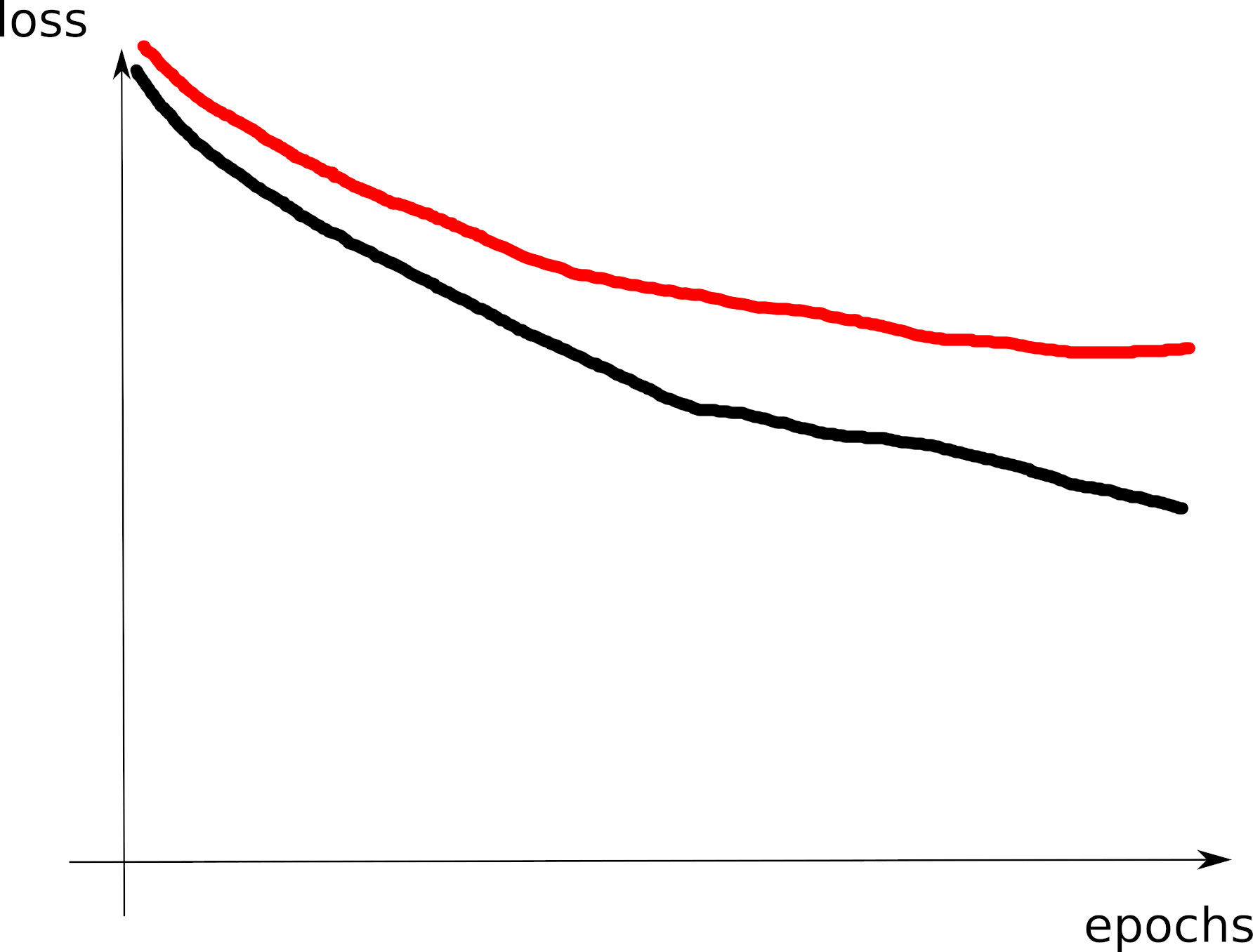
Curve 6
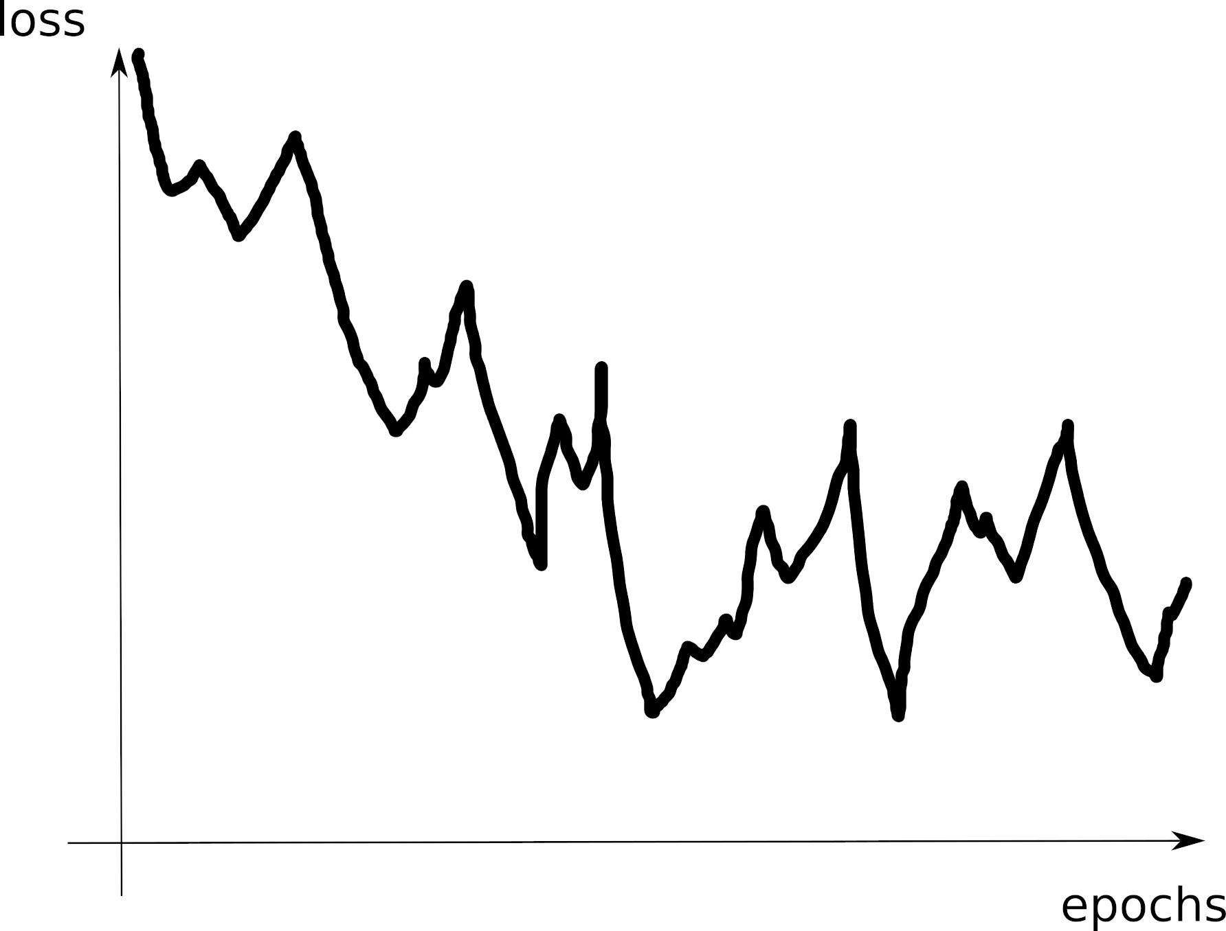
Curve 7
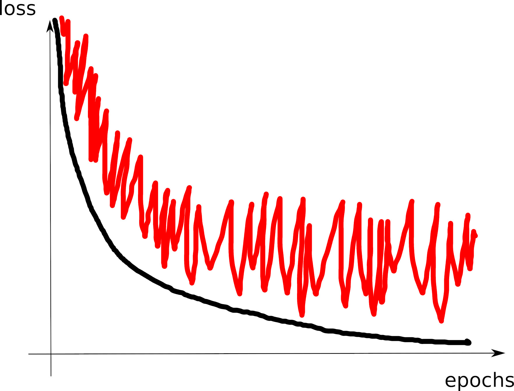
Curve 8
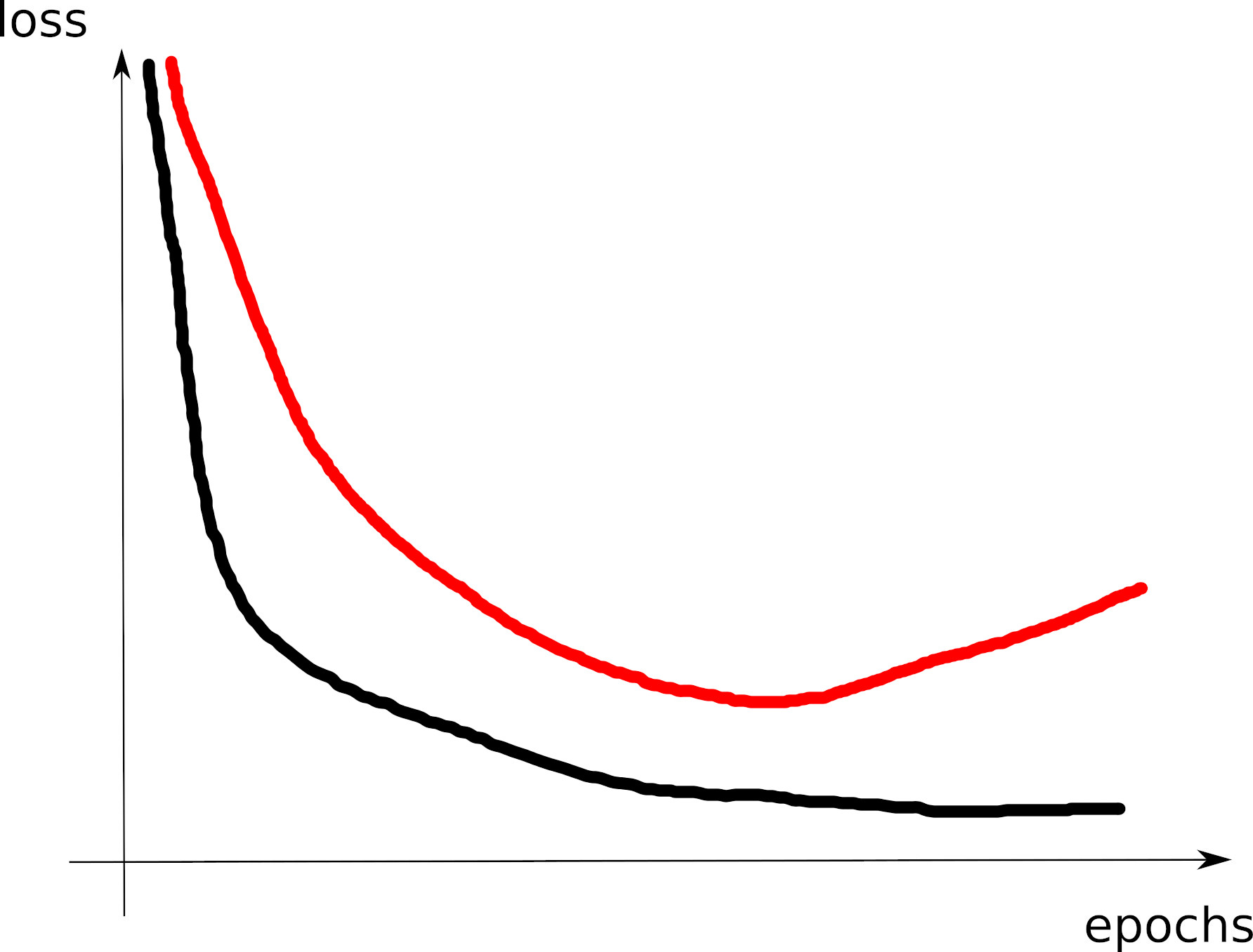
Visible effects
- Learning rate too large
- Learning rate too small
- Training loss not averaged enough
- Training and val losses not comparable
- Overfitting
- Underfitting
- Training too short / Convergence too slow
- Grokking
- \(x\perp\!\!\!\!\perp y\) (bug? bad data? ill-posed problem?)
- no shuffling of training set
- mismatch of train and val distributions
- spikes in gradients (LR or optimization issues)
- too much variability across runs (saddle? init?)
- not enough variability across runs (seed issue?)
- saddle point ? (multiple runs plateau at various levels)
- pretraining instabilities: tune weights initialization
- not enough regularization
- too much regularization
- exploding / vanishing gradients
- ill-conditioning of Hessian \(\rightarrow\) sharp valleys (see next)
Debugging a training
https://blog.slavv.com/37-reasons-why-your-neural-network-is-not-working-4020854bd607
- Check 1: Ensure your training loss is decreasing well
- Fast enough
- But not too fast
- Getting close enough to zero
- Without too many instabilities
- Without too much variability
- Can the training loss increase?
- Yes, but not too much and not too often!
- Can the training loss plateau?
- Yes, especially at the end and with a low-loss plateau
- If the plateau is high/at the beginning, it’s a sign something may be wrong
- bug? data issue? optimizer (saddle points)?
- Decreasing by steps (stairs-like shape):
- Did you shuffle data at the start of every epoch?
- May be OK, but the task looks hard for this optimizer
- Variabilities:
- how many samples do you compute the training loss with?
- Instabilities:
- First try changing the learning rate
- Then change your random weights initialization!
- Adjust warm-up, LR scheduler
Safety checks
- Good training loss curve:
- Starts high, decrease very fast at the start
- Then slows down its decrease
- Then regular and slow decrease (plateau down)
- Check 2: ensure your validation loss decreases
- similar or slightly higher values than train loss when computed the same ways
- good curve = U-shape, with moderate increase on the right
- Warning: validation data must be carefully chosen!
- shall represent the target generalization you are interested in
- cross-validation is often wrong:
- e.g.: you train your model in 2024, and want to deploy it in 2025
- target generalization = “work in the future”
- so you shall split your data: train = past data, validation = most recent data
- Check in order:
- the training + validation loss curves
- the gradient norm
- the weights distribution should be approximately gaussian after some time
- the updates distribution should also be gaussian
- the activations norm per layer
- What error/risk/loss shall you expect?
- depends on the task definition, the data available, the chosen model
- scaling laws = empirical functions that relate the model capacity to its error on a given task
- rules: the largest models always have largest capacity and better performance
- choose the largest model you can handle
- See normal LLM pretraining curves
- You may exploit scaling laws to detect issues with your data/task definition:
- train very small model, then retrain by progressively increasing size
- you should see an increase in performance
- otherwise: red flag (bug? task definition? data?)
- Same test can be made with data:
- also have their scaling laws
- same conclusion: the largest datasets always give better performances
- train model on very small data, then increase data size
- These checks also help in tuning hyperparameters, by giving you a sense of how the model react to more data/size
(Practical exo1)
Typical issues with validation loss
- does not decrease
- data issues: empty data, unrelated data, badly formatted, wrong data…
- optimizer issues: converges too fast, too slow
- validation curve perfectly matches training curve
- underfitting
- you really should try increasing your model size until you observe overfitting
- and then, may be, slightly reduce its capacity
- training loss goes to zero, but validation loss stays large
- overfitting: it’s OK to overfit:
- check the real impact on final metric
- add L2 regularization if it’s not good
- generalization gap
- you test data is too different from your train data?
- overfitting: it’s OK to overfit:
Less common things that may go wrong
- vanishing / exploding gradients
- may appear in deep and recurrent models
- Gradients may vanish because of non-linear activations
- may be detected by tracking gradient norms or parameter updates in each layer
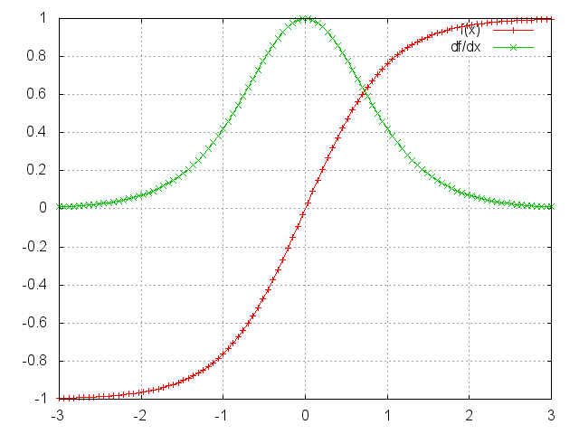
- Solutions for vanishing gradients:
- ReLU (or more recent: SwiGLU…) activations
- Skip connections
- Better initialization
- Exploding gradients: check gradient norm
- sudden jump in the training loss: may be due to a “cliff” in loss landscape, with very large gradients resulting in large jumps (see paper )
- compare the gradient norm with parameter norm:
- grad norm is proportional to parm norm
- so it’s OK that grad norm increases when parm norm increases as well
- Saddle points
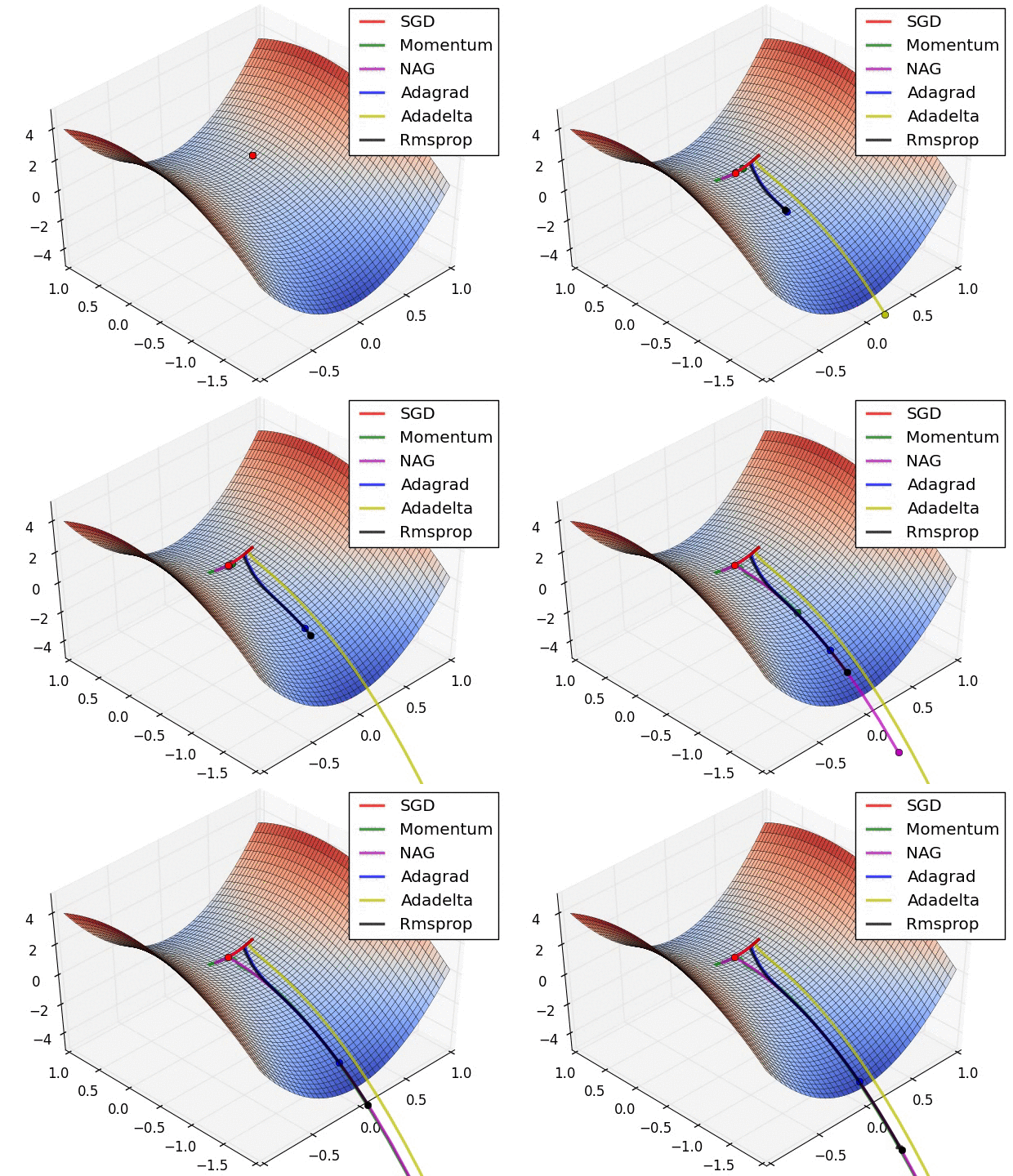
- Solutions against saddle points:
- try other optimizers (Adam, Adagrad, RMSProp… family)
- LR scheduler
- Batch norm: smooths loss landscape
- Noise injection
- Tracking weights change:
- Large weights change is normal for rare words with Adam
- Track variance of gradient mini-batch:
- large spike at 0, small elsewhere: vanishing gradient
- bimodal, too flat, not centered distribution: exploding gradient
- solved with batch norm, gradient clipping
- correlation traps
- If the activations in one layer become close to 0, very slow training in the deepest layers
- see Glorot paper
- momentum, ill-conditioning: see blog
- momentum speeds-up SGD quadratically
- ill-conditioned Hessian = curvature much larger in one dim than in another => sharp valley
- SGD will “bounce” between walls of this sharp valley
Loss landscape
- In the loss landscape:
- minima are connected together through “valleys”
- all local minima are also global minima
- See Kawaguchi
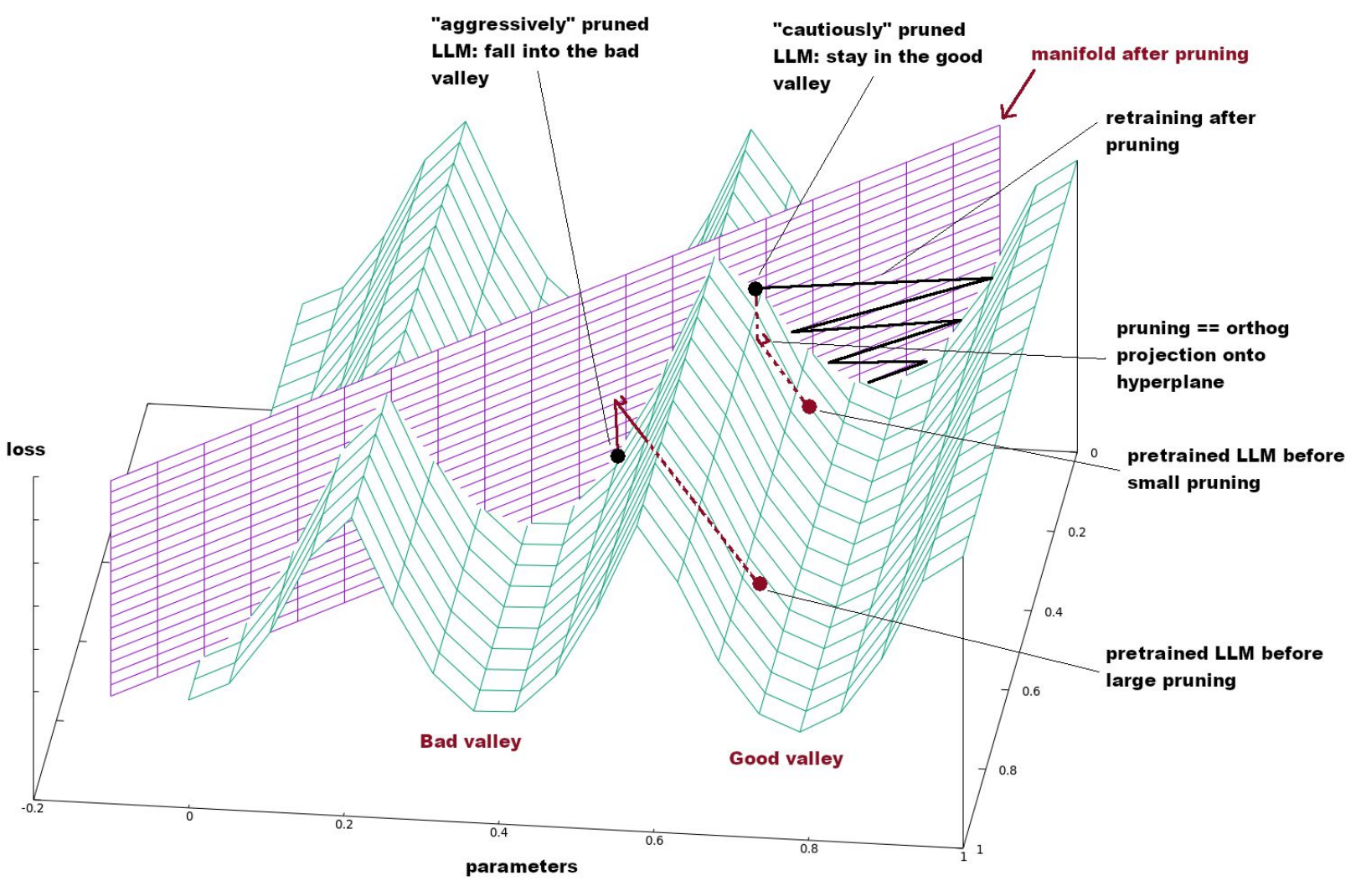
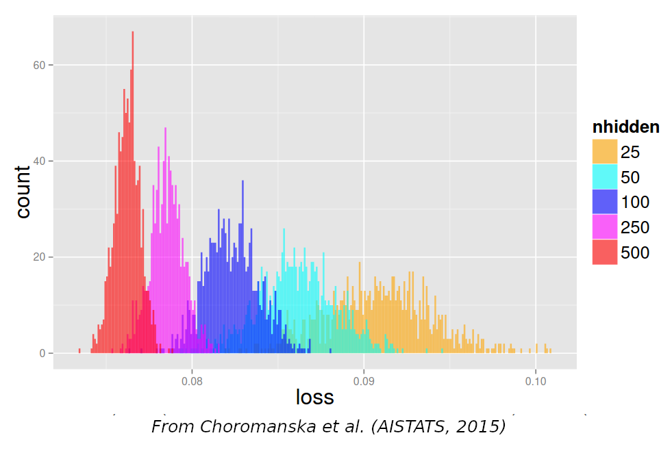
- Understanding the loss landscape is useful for:
- Optimizers: Adam, saddle points…
- Model merging: linearly connected models
- SGD convergence: edges, flatness
- Pruning, compression:
- Why iterative pruning?
- Why is calibration data required?
- …
On Bayes Risk and task definition
- Bayes risk = minimum erreur that is doable by an ideal model
- It depends on the way you formulate your task:
- input = time of day, output = month
- input = number, output = inverse of this number
- task definition:
- input = month, output = temperature
- Your minimal error is large!
- But you can do better by adding context:
- input = hour + month, output = temperature
- If your training loss plateaus too high, try adding context
- It’s good to have the training loss goes down to 0
Debugging process
- When something goes wrong:
- observe, collect various information, analyze
- make an hypothesis about what can go wrong
- make a test to validate your hypothesis
- What if you don’t have any hypothesis of what can go wrong?
- Test the most common causes of errors:
- Number 1 issue: bug in code/data processing
- First sanity test: make your model overfit on one batch
- Then progressively increase and adjust hyper-parms at the same time
- If you only tune 1 hyper-parm, you must tune the learning rate!
- Often, you just don’t train long enough…
- Test the most common causes of errors:
- Test the most common causes of errors:
- check your model:
- Simplify your model/code at the maximum: remove all options, use the simplest training loop possible, etc.
- print all intermediary results: are they expected ? No NaN, inf, too large value?
- replace your model with a simple SVM/…
- check your model:
- check your data:
- print the data at various parts of your code: is it still what you expect?
- change your data (replace some dimension, swith vectors…): are values the same, different?
- replace your input data with random noise, see if things run as expected
- replace your input with artificial data you control for each class
- is the dataset large enough?
- how many examples for each label do you have?
- did you normalize you data?
- did you shuffle your training corpus?
- Test the most common causes of errors:
- check your task:
- simplify your task: remove features, context, labels…
- what is the expected random accuracy?
- check your task:
- Collect more evidence, ask someone, ask chatgptb
- What if all curves look kinda OK?
- Don’t believe it!
- Make some more tests in different conditions
- You must progressively build up trust in your code, and only when you really trust your code, you can ship it
Practical session
- Inputs = capteurs de temp/pression, valeurs normalisees, sur un laminage de fer à haute température; 1 mesure par barre de fer
- Sortie = qualité du fer (OK / BAD) mesuré après refroidissement, 1 jour plus tard
- But = prédire la qualite
- fichier data: https://olki.loria.fr/cerisara/lexres/ferdata.csv
- TODO:
- train and evaluate a model: what is your accuracy?
Exo 2
- goal: train a classifier on 12 classes (imbalanced)
- download data from https://olki.loria.fr/cerisara/lexres/dataclas.txt
- Each line contains 1 sample, with features separated by white space
- Each line contains first the gold class (from 0 to 11), followed by this sample obs (10-dim vector)
- The following code trains an MLP on this data:
import torch
import torch.nn as nn

class Mdata(torch.utils.data.Dataset):
    def __init__(self):
        self.x = []
        self.y = []
        with open("dataclas.txt","r") as f:
            for l in f:
                ll = l.split(" ")
                self.y.append(torch.Tensor([int(ll[0])]))
                self.x.append(torch.Tensor([float(z) for z in ll[1:]]))

    def __getitem__(self,i):
        return self.x[i], self.y[i]

    def __len__(self):
        return len(self.x)

data = Mdata()
datal = torch.utils.data.DataLoader(data, batch_size=1, shuffle=True)

layers = []
layers.append(nn.Linear(10,20))
layers.append(nn.Sigmoid())
layers.append(nn.Linear(20,100))
mod = nn.Sequential(*layers)

def train():
    mod.train()
    floss = nn.CrossEntropyLoss()
    opt = torch.optim.SGD(mod.parameters(), lr=0.001)
    for ep in range(100):
        totloss = 0.
        for x,y in datal:
            ypred = mod(x)
            loss = floss(ypred,y)
            totloss += loss.item()
            loss.backward()
            opt.step()
        print("loss",ep,totloss)

train()

# This code contains exactly 3 bugs: find them and fix them!- TODO:
- copy-paste this code and debug it
- runs the training and observe the training curve: what happens?
(slides to delete - don’t read)
TODO: detecter:
serie temp tres longue avec dependance tres lointaine..
transf 1000 layers.. vanishing grad
data high dim steps like .. saddle points
dble descente
Randomness and noise
- Uncertainty: from the data vs. from the model
- estimating output distributions: DMN, bayesian inference
- multiple runs
- ensembling
- conformal predictions
- Random seeds
- shall we use seeds or not?
- yes for debugging
- no for evaluation
- practical concerns with seeds
- shall we use seeds or not?
- Various types of “noise”:
- data sampling noise = not the true distrib = pb of generalization
- quantization noise = noise on parameters
- regularization noise = during training
- dropout
- estimates of metrics: confidence intervals
- “noise in ouputs” = variety in generation:
- sampling
- beamsearch, greedy, global vs. local generation
- personas